by Rajat Jindal | May 21, 2026 | AWS
The Richest Data Source You Are Not Feeding to AI
Every enterprise AI initiative starts with the same discovery: “What data do we have that could power this?” The team surveys CRM records, support tickets, product documentation, customer emails. They build Knowledge Bases, generate embeddings, and deploy copilots.
But there is one system — the one that contains the most valuable structured business data in the organisation — that is almost never connected to AI in the first wave. It is your SAP ERP.
SAP holds the ground truth of your business: every purchase order, every invoice, every goods receipt, every vendor payment, every production order, every financial posting. It is the system of record for procurement, finance, supply chain, manufacturing, and HR. It contains ten years of transactional history that no other system in your enterprise possesses.
And yet, in my presales engagements across dozens of enterprise AI initiatives, SAP data is consistently the last to be connected — if it is connected at all. The reasons are always the same: “SAP is too complex,” “the ERP team will never approve it,” “we don’t know how to extract data from SAP safely.”
These objections are real but solvable. And the enterprises that solve them first will have an AI advantage that no competitor can replicate — because no competitor has their SAP transaction history.
This post is about why SAP data is the highest-value AI data source in the enterprise, how to connect it to AWS AI services without disrupting your ERP, and the business outcomes that become possible when your AI can finally answer questions that only SAP knows the answer to.
Why SAP Data Is Different: The Unique AI Value Proposition
Other Systems Tell You What People Said. SAP Tells You What Actually Happened.
CRM data tells you what a salesperson recorded about a customer conversation. Support tickets tell you what a customer described as their problem. Emails tell you what people promised each other.
SAP tells you what actually happened: the purchase order that was raised, the goods that were received, the invoice that was matched, the payment that cleared. It is the financial and operational ground truth — not a record of intentions, but a record of actions.
For AI, this distinction is transformative. An AI grounded in SAP data does not hallucinate about business performance — it reports what actually occurred, with document numbers, timestamps, and financial amounts that tie back to auditable transactions.
The Data Moat
Every enterprise has access to the same foundation models. Every enterprise can build a chatbot. The differentiator is not the AI — it is the data the AI has access to.
SAP data is the ultimate proprietary data moat:
- Your vendor payment history is uniquely yours
- Your procurement patterns are competitively sensitive
- Your production efficiency data reflects your specific operations
- Your financial transaction history tells the real story of your business
An AI connected to this data can answer questions that no public AI tool, no competitor, and no generic analytics platform can answer. That is the competitive advantage — and it compounds with every month of transaction history.
The Three Barriers (and How AWS Solves Each One)
The reality: SAP’s data model is complex — normalised across hundreds of tables with cryptic naming conventions (VBAK, EKPO, BSEG, MSEG). Extracting meaningful data historically required deep ABAP expertise and months of development.
The AWS solution: Amazon AppFlow provides native SAP connectors that extract data from SAP without ABAP development, without impacting ERP performance, and without exposing the underlying table complexity to downstream systems.
{
  "flowName": "sap-procurement-to-s3",
  "description": "Extract procurement data from SAP for AI consumption",
  "sourceFlowConfig": {
    "connectorType": "SAPOData",
    "connectorProfileName": "sap-s4hana-production",
    "sourceConnectorProperties": {
      "SAPOData": {
        "objectPath": "/sap/opu/odata/sap/API_PURCHASEORDER_PROCESS_SRV/A_PurchaseOrder",
        "paginationConfig": {
          "maxPageSize": 5000
        }
      }
    }
  },
  "destinationFlowConfig": [
    {
      "connectorType": "S3",
      "destinationConnectorProperties": {
        "S3": {
          "bucketName": "enterprise-data-lake",
          "bucketPrefix": "sap/procurement/purchase-orders/",
          "s3OutputFormatConfig": {
            "fileType": "PARQUET",
            "prefixConfig": {
              "prefixType": "PATH_AND_FILENAME",
              "prefixFormat": "YEAR/MONTH/DAY"
            }
          }
        }
      }
    }
  ],
  "triggerConfig": {
    "triggerType": "Scheduled",
    "triggerProperties": {
      "scheduleExpression": "rate(1day)",
      "dataPullMode": "Incremental",
      "scheduleStartTime": "2026-05-01T02:00:00Z"
    }
  }
}
The key architectural decision: incremental extraction on a schedule rather than bulk extraction. AppFlow pulls only changed records since the last run, keeping data fresh without overloading the SAP system. The ERP team’s concern — “extraction will degrade our production system” — is addressed by design.
Barrier 2: “The ERP Team Will Never Approve Access”
The reality: SAP teams are protective of their system — and rightfully so. ERP downtime is a business-stopping event. Any integration that risks performance or data integrity will be blocked.
The AWS solution: The extraction architecture operates through SAP’s OData APIs — the same API layer SAP itself provides for external integrations. It does not require direct database access, ABAP development, or changes to the SAP system. The SAP team approves an API user with read-only access to specific OData services — nothing more.
The governance conversation that works with ERP teams:
- Read-only access (no write-back to SAP)
- API-level extraction (no database-level queries)
- Scheduled during off-peak hours (configurable in AppFlow)
- Specific entity access only (not “all SAP data”)
- Full CloudTrail audit logging of every extraction
When framed this way — as a read-only, API-based, audited, scheduled extraction — the approval conversation shifts from “no” to “which entities do you need?”
Barrier 3: “We Don’t Know How to Make SAP Data AI-Consumable”
The reality: SAP data is heavily structured — transaction codes, document numbers, currency amounts, material numbers. AI models expect natural language or semantically meaningful text. The gap between SAP’s structured format and AI’s consumption expectations is real.
The AWS solution: A transformation layer that converts structured SAP transactions into semantically meaningful text for embedding and AI consumption — while preserving the structured data for analytics.
# Glue ETL: Transform SAP procurement data into AI-consumable format
import boto3
from awsglue.context import GlueContext
from pyspark.context import SparkContext
from pyspark.sql.functions import concat_ws, col, lit, when

sc = SparkContext()
glueContext = GlueContext(sc)

# Read SAP purchase orders from S3 (landed by AppFlow)
po_data = glueContext.create_dynamic_frame.from_catalog(
    database="sap_data_lake",
    table_name="purchase_orders"
).toDF()

# Transform structured SAP data into semantic text for AI embedding
ai_ready = po_data.withColumn(
    "semantic_text",
    concat_ws(" ",
        lit("Purchase Order"),
        col("PurchaseOrder"),
        lit("was created on"),
        col("CreationDate"),
        lit("for vendor"),
        col("Supplier_Name"),
        lit("with total value"),
        col("PurchaseOrderNetAmount"),
        col("DocumentCurrency"),
        lit("containing"),
        col("NumberOfItems"),
        lit("line items for material group"),
        col("MaterialGroup_Description"),
        lit("with delivery date"),
        col("DeliveryDate"),
        lit("and current status"),
        when(col("PurchasingProcessingStatus") == "02", lit("Approved"))
        .when(col("PurchasingProcessingStatus") == "04", lit("Goods Received"))
        .when(col("PurchasingProcessingStatus") == "06", lit("Invoice Received"))
        .otherwise(lit("In Progress"))
    )
)

# Write both formats:
# 1. Parquet (structured) — for analytics, Athena, Redshift
# 2. Semantic text — for Bedrock Knowledge Base, embeddings

# Structured for analytics
glueContext.write_dynamic_frame.from_options(
    frame=DynamicFrame.fromDF(ai_ready, glueContext, "ai_ready"),
    connection_type="s3",
    connection_options={"path": "s3://enterprise-data-lake/sap/ai-ready/procurement/"},
    format="parquet"
)
The dual-write pattern is the key design decision: the same data is available in structured format (for SQL analytics) and semantic format (for AI consumption). One extraction, two consumption patterns.
What Becomes Possible: AI Use Cases Powered by SAP Data
Once SAP data flows into your AWS AI platform, use cases that were previously impossible — or required weeks of manual analysis — become instant:
Use Case 1: Intelligent Procurement Insights
The question: “Which vendors have the highest rejection rates, and what is the financial impact of switching to alternatives?”
Without SAP-AI integration: A procurement analyst spends 2-3 days extracting data from SAP, building Excel models, cross-referencing quality records, and preparing a recommendation deck.
With SAP-AI integration: A Bedrock agent connected to SAP procurement history answers in seconds — grounded in actual goods receipt records, quality inspection results, and payment history spanning years.
Use Case 2: Cash Flow Forecasting
The question: “Based on our current open purchase orders, goods receipts pending invoice, and historical payment patterns, what is our expected cash outflow for the next 30/60/90 days?”
Without SAP-AI integration: Finance team manually runs SAP reports (ME2M, FBL1N), exports to Excel, applies assumptions, and builds a forecast. Takes 1-2 days each cycle.
With SAP-AI integration: An AI agent queries open PO data, historical payment terms compliance by vendor, and seasonal patterns — delivering a forecast in real-time that updates as new transactions post.
Use Case 3: Supplier Risk Early Warning
The question: “Are any of our critical suppliers showing patterns that indicate financial stress or delivery reliability issues?”
Without SAP-AI integration: Reactive — you discover supplier problems when deliveries are late or quality declines.
With SAP-AI integration: An AI agent monitors SAP transaction patterns continuously — increasing lead times, changing payment term requests, declining quality inspection pass rates — and alerts procurement before the risk materialises.
Use Case 4: Natural Language SAP Queries for Non-Technical Users
The question: Finance director asks “How much did we spend on logistics services in Q1 versus Q1 last year?”
Without SAP-AI integration: The finance director submits a request to the SAP reporting team, waits 2-3 days for a custom report.
With SAP-AI integration: Amazon Q Business, connected to SAP financial data in S3, answers the question immediately — in natural language, with source citations back to specific SAP document numbers.
The Architecture: SAP → AWS → AI
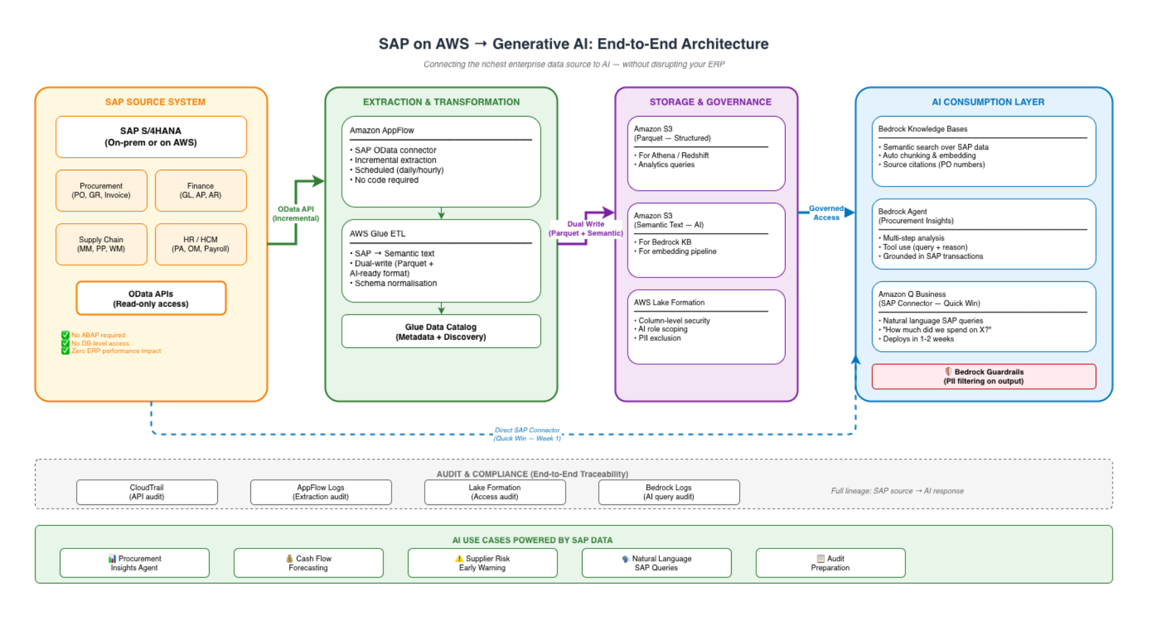
Amazon Q Business: The Quick Win
Amazon Q Business has a native SAP connector — meaning you can connect Q Business to SAP without building the full extraction pipeline first. For organisations wanting immediate value, Q Business provides natural language access to SAP data within weeks, not months.
The trade-off: Q Business provides conversational access but limited customisation. For advanced use cases (agents with tool use, custom reasoning, multi-step analysis), the full pipeline (AppFlow → S3 → Bedrock Knowledge Base → Bedrock Agent) gives you maximum flexibility.
My recommendation: Deploy Q Business with the SAP connector as Week 1 value demonstration. Build the full pipeline in parallel for advanced use cases. This gives stakeholders immediate evidence of AI-over-SAP value while the engineering team builds the production architecture.
The Business Case: SAP-AI Integration Economics
What Changes When AI Can Query SAP
| Business Function |
Current State (Manual) |
AI-Enabled State |
Time Savings |
| Procurement analysis |
2-3 days per report |
Real-time agent response |
90%+ |
| Cash flow forecasting |
1-2 days per cycle |
Continuous, auto-updating |
85%+ |
| Vendor performance review |
Quarterly (manual compilation) |
Continuous monitoring with alerts |
From reactive to proactive |
| Ad-hoc SAP queries |
2-3 day turnaround from SAP team |
Instant via Q Business |
95%+ |
| Audit preparation |
2-4 weeks |
Days (AI retrieves evidence instantly) |
80%+ |
Implementation Cost
| Component |
Cost |
Timeline |
| AppFlow SAP connector setup |
$5K-$15K |
1-2 weeks |
| Glue ETL for AI transformation |
$10K-$25K |
2-3 weeks |
| Bedrock Knowledge Base on SAP data |
$5K-$10K |
1 week |
| Q Business with SAP connector |
$20/user/month |
1-2 weeks |
| Lake Formation governance |
$10K-$20K |
2-3 weeks |
| Total initial investment |
$30K-$70K |
6-10 weeks |
ROI Drivers
- Procurement team productivity: 2-3 analysts each saving 1-2 days/week on manual SAP reporting = $60K-$80K/year in recovered capacity
- Faster decision-making: Cash flow forecasts available daily instead of monthly = better working capital management
- Risk avoidance: Early supplier risk detection prevents supply chain disruptions ($50K-$150K per incident avoided)
- Audit efficiency: 80% reduction in audit preparation time = $20K-$40K/year
Typical first-year ROI: 2-3x the initial investment — driven primarily by the productivity gains of giving finance and procurement teams natural language access to data they currently wait days to receive.
A Presales Perspective: Positioning SAP-AI in Customer Conversations
Why This Conversation Is Uniquely Powerful
Most AI presales conversations compete with dozens of other vendors offering generic AI capabilities. The SAP-AI conversation has no competition — because it requires specific expertise that few partners possess:
- Deep SAP knowledge — understanding the data model, OData services, extraction patterns
- AWS AI expertise — Bedrock, Knowledge Bases, Q Business, AppFlow
- Enterprise integration experience — governance, security, performance considerations
Partners who can credibly deliver all three are rare. That scarcity is the positioning advantage.
The Opening Question
“Your SAP system contains ten years of procurement, financial, and operational transaction data. Today, how long does it take someone in finance or procurement to get an answer from that data?”
The answer is always “days” or “we have to ask the SAP team.” That gap — between the value of the data and the accessibility of it — is the opportunity.
The Demonstration That Wins
Show Q Business answering a question about the customer’s own SAP data (in a demo environment): “What were our top 10 vendors by spend last quarter, and which of them had delivery delays exceeding 5 days?”
When a CFO sees that question answered in 3 seconds instead of 3 days, the business case conversation is over. The only remaining question is timeline.
The Objection You Will Hear
“We’re planning to move to S/4HANA — shouldn’t we wait?”
Response: “The AI platform we build today works identically whether your SAP is ECC or S/4HANA. AppFlow connects to both via OData. If anything, building AI-over-SAP now gives you a compelling reason to accelerate the S/4HANA migration — because S/4HANA’s improved APIs make AI integration even simpler. You are not building throwaway work — you are building the AI layer that survives the migration.”
Governance: What the CISO Needs to Hear
SAP data is among the most sensitive in the enterprise — financial records, vendor contracts, employee information. The CISO will rightfully scrutinize any AI system that touches it.
The governance architecture that addresses their concerns:
- Read-only extraction: AppFlow pulls data via OData with a service account that has zero write permissions in SAP. The AI can never modify ERP data.
- Lake Formation scoping: The AI service role sees only approved SAP entities — purchase orders and vendor master, for example — not HR compensation or financial postings.
- Column exclusion: Sensitive fields (bank account numbers, personal IDs, salary data) are excluded at the Glue transformation layer — they never enter the AI-accessible S3 path.
- Bedrock Guardrails: Output-layer protection ensures the AI does not surface financial amounts or vendor names that the requesting user is not authorised to see.
- Full audit trail: CloudTrail logs every AppFlow extraction, every Bedrock query, every S3 access — creating a complete lineage from SAP source to AI response.
The message: “The AI has less access to SAP data than your average SAP power user. It sees a governed subset, it can only read, and every access is logged.”
Lessons for Technology Leaders
- Your ERP is your AI moat — but only if you connect it — Every competitor has access to the same foundation models. None of them have your SAP transaction history. The enterprise that connects AI to SAP data first builds an insight advantage that compounds with every month of history.
- Start with Q Business for quick wins, build the full pipeline for advanced use cases — Q Business with the SAP connector demonstrates value in weeks. The full architecture (AppFlow → S3 → Bedrock) enables agent-level AI that Q Business alone cannot deliver. Run both in parallel.
- The SAP team is an ally, not a blocker — frame it correctly — Read-only API access, scheduled off-peak, specific entities only, fully audited. When framed as “we need to read purchase orders via OData,” the conversation is straightforward. When framed as “we need access to SAP,” it sounds terrifying. Language matters.
- Dual-write architecture serves both analytics and AI — The same extraction pipeline feeds structured data (for Athena/Redshift analytics) and semantic data (for Bedrock AI). One investment, two value streams.
- SAP-AI integration is a rare skill combination — and a presales differentiator — Most AWS partners cannot credibly deliver SAP + AI. Most SAP partners cannot credibly deliver AWS AI. The partner that delivers both wins deals that neither competitor can contest. That intersection is where the highest-value enterprise conversations happen.
About the Author
Rajat Jindal is VP – Presales at AeonX Digital Technology Limited, where he architects winning cloud strategies for enterprise customers and translates modernization into measurable business value. He is a strong advocate of AWS, committed to sharing thought leadership that helps technology leaders make faster, better-informed decisions.
by Chandni Gadhvi | May 13, 2026 | AWS
The Sprawl Problem: Why Letting Every Team Build Their Own Bedrock Integration Is a Mistake
When Amazon Bedrock became available in India regions, the reaction across our enterprise client's five business units was predictable and immediate. The CRM team wanted it for customer email drafting. The finance team wanted it for contract summarization. The HR team wanted it for policy Q&A. The supply chain team wanted it for procurement intelligence. The product team wanted it for release note generation.
Within three months, each team had independently built their own Bedrock integration. Five separate boto3 clients. Five separate prompt templates with no shared standards. Five separate S3 buckets used as ad-hoc knowledge sources. No visibility into what any team was spending. No audit trail that compliance could use. No way to enforce the data access rules that said the HR team's knowledge base should never be queryable by the supply chain team. And no shared learning — if the CRM team figured out a better prompting pattern, the finance team had no way to know.
This is the pattern that emerges when AI adoption is driven bottom-up without a central integration layer. It is not a failure of the teams — each integration worked. It is a failure of architecture. Five teams solved the same problem five times, created five separate cost centres that finance could not track, built five separate security postures that varied in quality, and accumulated five sets of technical debt that would compound with every new model version and every new use case.
Within those five integrations, the same problems existed independently: hardcoded model IDs that would break on deprecation, no prompt injection protection, and five separate OpenSearch Serverless collections costing a combined $1,752/month for knowledge bases that collectively held fewer than 25,000 documents.
The question was not whether to consolidate — the business case was obvious. The question was how to build a centralized Bedrock gateway that felt invisible to each team: same latency, same flexibility, same ability to customize prompts and knowledge sources — but with tenant isolation, cost attribution, token budget enforcement, and a unified audit trail baked in at the infrastructure layer.
This post documents that architecture.
As Technical Architect for this initiative at AeonX Digital, I designed the gateway, defined the tenant isolation model, and worked with each business unit's team through the migration from their independent integrations. What follows covers the implementation decisions, the security trade-offs, and the operational patterns that make a shared AI gateway work without becoming a bottleneck.
The outcome: total AI infrastructure spend reduced from $3,093/month to $936/month, three compliance findings closed, and five teams freed from maintaining independent Bedrock integrations.
Why This Matters Now: The Enterprise AI Governance Inflection Point
Three forces are pushing enterprises from ad-hoc AI integrations toward centralized AI infrastructure:
- AI spend is becoming material and invisible simultaneously — At small scale, individual Bedrock integrations are cheap enough that nobody notices. As usage grows, the aggregate spend becomes significant — but because it is distributed across multiple cost centres with no tagging discipline, no single owner can see the full picture. Finance starts asking questions nobody can answer. Centralizing the integration makes AI spend visible and attributable before it becomes a governance problem.
- Data isolation is a legal requirement, not a preference — An enterprise running HR, finance, and customer data through AI systems has legal and contractual obligations about which data can be processed alongside which other data. Five independent integrations mean five independent security reviews, five sets of IAM policies to audit, and five potential misconfiguration surfaces. A single gateway with tenant isolation enforced at the infrastructure layer reduces that attack surface to one.
- Prompt and model governance cannot scale team-by-team — When a new Claude model version is released, or when a prompt injection pattern is identified as a security risk, updating five independent integrations requires coordinating five teams on their own timelines. A centralized gateway means one update propagates to all tenants simultaneously, with no individual team dependency.
The decision to build this gateway was driven by a CTO who had approved five separate AI initiatives, received five separate invoices he could not reconcile, and recognized that the architecture needed to evolve before the tenth initiative was approved.
The Business Problem
The enterprise's five-team AI sprawl produced:
- No unified cost visibility — Bedrock spend split across five cost centres with no consistent tagging, making total AI infrastructure cost impossible to report accurately
- No cross-tenant data isolation enforcement — each team's knowledge base was accessible to any team with valid AWS credentials, relying on convention rather than controls
- No token budget enforcement — one team's batch summarization job consumed 4× its expected token volume in a single week, approaching the account's Bedrock service quota and disrupting other teams' real-time use
- No unified audit trail — compliance could not produce a complete record of what data had been processed by AI systems, which models had been used, or what outputs had been generated
- Duplicated and expensive infrastructure — five separate OpenSearch Serverless collections for knowledge bases that could have shared a single collection with namespace isolation
Business impact:
- CFO unable to attribute AI infrastructure cost to individual business units for budget accountability
- Three open compliance findings related to AI data handling and audit traceability
- One quota throttling incident that disrupted two teams' real-time applications during a peak business period
- Engineering time duplicated across five teams solving identical infrastructure problems independently
The goal was a gateway that was invisible in normal operation — same API contract, same flexibility for each team — but that enforced isolation, attribution, and governance as infrastructure rather than convention.
Technical Architecture
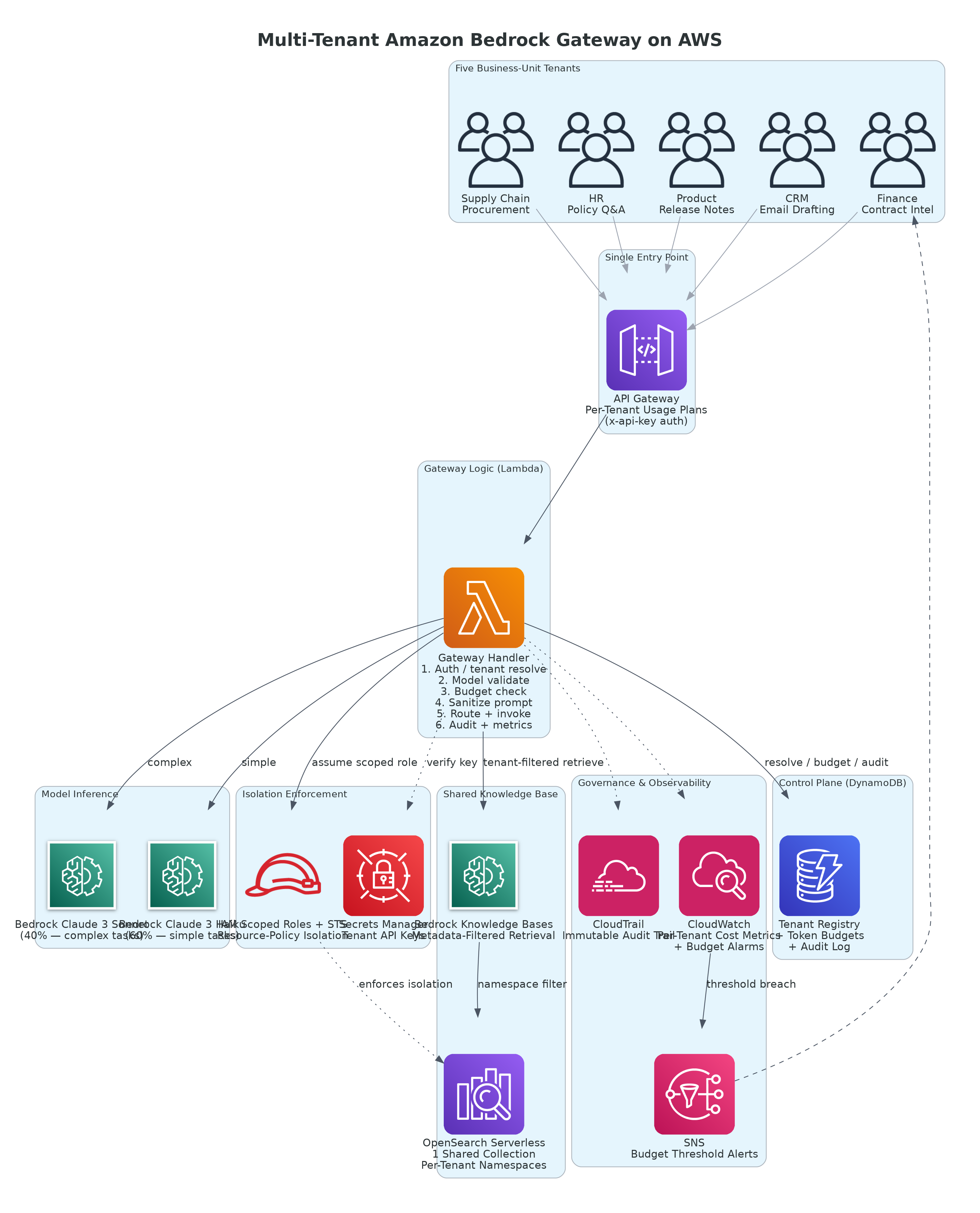
Figure 1: Multi-Tenant Amazon Bedrock Gateway — Centralized Integration Serving Five Business Units
AWS Services Used:
- Amazon API Gateway — single HTTPS entry point for all tenant requests with per-route usage plans
- AWS Lambda — gateway logic: authentication, tenant resolution, budget enforcement, model routing, audit logging
- Amazon Bedrock — foundation model inference (Claude 3 Sonnet for complex tasks, Claude 3 Haiku for simple classification and drafting)
- Amazon Bedrock Knowledge Bases — per-tenant logical isolation within a single shared OpenSearch Serverless collection using metadata filters
- Amazon OpenSearch Serverless — single shared vector search collection with per-tenant index namespaces
- Amazon DynamoDB — tenant registry, daily token budget state, and request audit log
- AWS IAM and AWS STS — execution roles with scoped assume-role for knowledge base access enforcement
- Amazon CloudWatch — request metrics, budget utilization dashboards, anomaly detection on usage patterns
- AWS CloudTrail — immutable API-level audit trail for compliance
- Amazon SNS — budget threshold alerts to tenant owners and platform team
- AWS Secrets Manager — tenant API key storage
The gateway sits between every tenant application and Amazon Bedrock. No tenant calls Bedrock directly. All requests flow through the gateway, which handles authentication, budget checking, model routing, and audit logging before the Bedrock call — and metric publishing after.
Key Architectural Decisions
These are the decisions that shaped the gateway — and the reasoning behind each one.
Decision 1: Why a Single AWS Account With IAM-Based Isolation Instead of One Account Per Tenant?
The first design question was account topology. Multi-account isolation — one AWS account per business unit — is the AWS Organizations best practice for the strongest boundary. It was also the option that would have taken three to four months to implement, required significant organizational change management, and introduced cross-account Bedrock quota management complexity that had no clean solution at the time of implementation.
We chose single-account with IAM-based isolation for reasons specific to this context:
| Approach |
Isolation Strength |
Implementation Time |
Operational Complexity |
| One account per BU |
Strongest — hard account boundary |
3–4 months |
High — cross-account routing, quota management per account |
| Single account, IAM role isolation |
Strong — enforced at resource policy level |
3–4 weeks |
Low — centralized management |
| Single account, application-layer isolation |
Weakest — relies on code correctness |
1–2 weeks |
Low — but misconfiguration creates data exposure risk |
The business decision: IAM resource policies on Bedrock Knowledge Bases enforce that the Lambda execution role scoped to Tenant A cannot invoke the knowledge base belonging to Tenant B — not because the code prevents it, but because the IAM policy denies it at the AWS API level. That is infrastructure-enforced isolation, not application-enforced isolation. For the data classification requirements in scope, it was sufficient — and deliverable in weeks rather than months.
Decision 2: Why One Shared OpenSearch Serverless Collection Instead of One Per Tenant?
The five independent integrations each had their own OpenSearch Serverless collection. The combined cost was $1,752/month ($350.40 per collection × 5), driven by OSS's minimum billing of two OCUs per collection regardless of actual document volume or query load.
We consolidated to a single shared collection with per-tenant namespace isolation: each tenant's documents are indexed with a tenant_id metadata field, and all knowledge base queries include a mandatory metadata filter that restricts retrieval to the requesting tenant's documents. The IAM policy on the collection denies retrieval requests that omit the tenant filter — ensuring isolation is enforced at the infrastructure layer, not just in application code.
Cost impact: one collection at the 2 OCU minimum ($350.40/month) versus five separate collections at $1,752/month — a saving of $1,401.60/month on knowledge base infrastructure alone.
The business decision: Logical namespace isolation with IAM-enforced metadata filtering provides equivalent data isolation to physical collection separation at 20% of the cost. For knowledge bases containing internal enterprise documents — not customer PII — it is the right trade-off.
Decision 3: Why Lambda Instead of Direct API Gateway to Bedrock Integration?
API Gateway supports direct service integrations — you can wire it to invoke Bedrock without a Lambda in the middle. It removes the Lambda cold start concern and reduces per-request cost. We chose Lambda because the direct integration cannot satisfy four specific requirements:
- Pre-request budget check — requires a DynamoDB read before the Bedrock call. The direct integration has no pre-call interception point.
- Dynamic model routing — routing simple tasks to Claude 3 Haiku and complex tasks to Claude 3 Sonnet based on a request-level complexity signal requires logic that cannot live in a mapping template.
- Post-response audit logging — writing actual token consumption from the Bedrock response to DynamoDB and CloudWatch requires post-call processing that the direct integration cannot do conditionally.
- Prompt sanitization — stripping system prompt override attempts before the request reaches Bedrock requires an interception layer.
At 180,000 requests per month with average duration of 2.8 seconds and 512MB memory, the Lambda compute stays well within the free tier's 400,000 GB-second monthly allocation. The Lambda cost for this gateway is effectively zero. The cold start concern for an internal enterprise tool — where occasional 400ms cold starts are acceptable — does not justify provisioned concurrency at $170/month.
The business decision: Lambda adds negligible cost at this request volume, fits entirely within the free tier, and enables four capabilities the direct integration cannot support. The trade-off is straightforward.
Implementation Pattern
Tenant Registry: DynamoDB Schema
The tenant registry is the source of truth for gateway configuration. Every inbound request resolves a tenant record before any processing occurs.
BASH
# Tenant registry record — DynamoDB Table: BedrockGatewayTenants
# PK: tenant_id  |  GSI: ApiKeyHashIndex on api_key_hash

{
    "tenant_id":        "BU-FINANCE",
    "tenant_name":      "Finance — Contract Intelligence",
    "api_key_hash":     "e3b0c44298fc1c149afb...sha256 of issued key",  # Never stored plaintext
    "status":           "ACTIVE",       # ACTIVE | SUSPENDED | RATE_LIMITED

    "allowed_models": [
        "anthropic.claude-3-sonnet-20240229-v1:0",
        "anthropic.claude-3-haiku-20240307-v1:0"
    ],

    # Knowledge base access — KB ID for metadata-filtered retrieval
    "kb_tenant_namespace": "finance",   # Used as metadata filter value in OSS queries

    # Token budget — reset daily at tenant's local midnight
    "daily_token_budget":  1_500_000,   # 1.5M tokens/day (realistic for contract summarization)
    "burst_limit_pct":     25,          # Max 25% of daily budget in any 15-min window
    "budget_alert_pct":    80,

    # Cost attribution — applied to CloudWatch metrics for cost reporting
    "cost_centre":     "CC-7821",
    "department":      "Finance",
    "budget_timezone": "Asia/Kolkata",  # Reset at midnight IST, not UTC

    "owner_email":     "finance-ai-owner@company.com",
    "alert_sns_arn":   "arn:aws:sns:ap-south-1:111122223333:finance-ai-alerts"
}
Gateway Lambda: Core Request Handler
PYTHON
import boto3, json, hashlib, time
from datetime import datetime, timezone
from botocore.exceptions import ClientError

dynamodb  = boto3.resource("dynamodb", region_name="ap-south-1")
bedrock   = boto3.client("bedrock-runtime", region_name="ap-south-1")
cw        = boto3.client("cloudwatch", region_name="ap-south-1")

tenant_table = dynamodb.Table("BedrockGatewayTenants")
budget_table = dynamodb.Table("BedrockTokenBudgets")
audit_table  = dynamodb.Table("BedrockAuditLog")

# In-memory tenant cache — avoids a DynamoDB read on every request
# Lambda execution environment persists across warm invocations
_tenant_cache: dict = {}

def lambda_handler(event, context):
    start_ms = time.time() * 1000

    # ── 1. Authenticate and resolve tenant ───────────────────────────────
    api_key = event.get("headers", {}).get("x-api-key", "")
    if not api_key:
        return _err(401, "Missing x-api-key header")

    tenant = _resolve_tenant(api_key)
    if not tenant:
        return _err(401, "Unrecognised API key")
    if tenant["status"] != "ACTIVE":
        return _err(403, f"Tenant account is {tenant['status']}")

    tenant_id = tenant["tenant_id"]
    body = json.loads(event.get("body") or "{}")

    # ── 2. Validate requested model ──────────────────────────────────────
    model_id = body.get("model_id")
    if not model_id or model_id not in tenant["allowed_models"]:
        return _err(403, f"Model '{model_id}' not permitted for this tenant")

    # ── 3. Budget check — atomic DynamoDB conditional update ─────────────
    messages  = body.get("messages", [])
    est_tokens = sum(len(m.get("content", "").split()) * 1.3 for m in messages)  # rough estimate
    budget_ok = _check_budget(tenant_id, int(est_tokens), tenant)
    if not budget_ok:
        _publish(tenant_id, tenant, "BudgetBlocked", 1)
        return _err(429,
            f"Daily token budget exhausted for {tenant_id}. "
            f"Resets at midnight {tenant['budget_timezone']}. "
            f"Contact {tenant['owner_email']} to request a limit increase.")

    # ── 4. Sanitize messages (strip prompt injection attempts) ───────────
    messages = _sanitize(messages)

    # ── 5. Build and dispatch Bedrock request ────────────────────────────
    bedrock_payload = {
        "anthropic_version": "bedrock-2023-05-31",
        "max_tokens": min(int(body.get("max_tokens", 1024)), 2048),
        "temperature": float(body.get("temperature", 0.3)),
        "messages": messages
    }

    # Inject knowledge base context if tenant has a namespace and request opts in
    if tenant.get("kb_tenant_namespace") and body.get("use_knowledge_base"):
        bedrock_payload = _inject_kb_context(
            bedrock_payload,
            namespace=tenant["kb_tenant_namespace"],
            query=messages[-1]["content"]
        )

    response = bedrock.invoke_model(
        modelId=model_id,
        contentType="application/json",
        accept="application/json",
        body=json.dumps(bedrock_payload)
    )
    result = json.loads(response["body"].read())

    # ── 6. Record actual token usage and publish metrics ─────────────────
    usage        = result.get("usage", {})
    input_tok    = usage.get("input_tokens", 0)
    output_tok   = usage.get("output_tokens", 0)
    latency_ms   = int(time.time() * 1000 - start_ms)

    _update_budget_actuals(tenant_id, input_tok + output_tok)
    _publish(tenant_id, tenant, "RequestCount",  1)
    _publish(tenant_id, tenant, "InputTokens",   input_tok)
    _publish(tenant_id, tenant, "OutputTokens",  output_tok)
    _publish(tenant_id, tenant, "LatencyMs",     latency_ms, unit="Milliseconds")

    audit_table.put_item(Item={
        "request_id":       context.aws_request_id,
        "tenant_id":        tenant_id,
        "model_id":         model_id,
        "input_tokens":     input_tok,
        "output_tokens":    output_tok,
        "latency_ms":       latency_ms,
        "used_kb":          bool(body.get("use_knowledge_base")),
        "timestamp":        datetime.now(timezone.utc).isoformat(),
        "ttl":              int(time.time()) + (90 * 86400)   # 90-day audit retention
    })

    return {"statusCode": 200, "body": json.dumps({
        "content":    result["content"],
        "usage":      usage,
        "request_id": context.aws_request_id
    })}


def _resolve_tenant(api_key: str) -> dict | None:
    key_hash = hashlib.sha256(api_key.encode()).hexdigest()
    if key_hash in _tenant_cache:
        return _tenant_cache[key_hash]
    result = tenant_table.query(
        IndexName="ApiKeyHashIndex",
        KeyConditionExpression="api_key_hash = :h",
        ExpressionAttributeValues={":h": key_hash}
    ).get("Items", [])
    tenant = result[0] if result else None
    if tenant:
        _tenant_cache[key_hash] = tenant   # Cache in warm Lambda memory
    return tenant


def _err(code: int, msg: str) -> dict:
    return {"statusCode": code, "body": json.dumps({"error": msg})}
Atomic Token Budget Enforcement
PYTHON
from decimal import Decimal
from boto3.dynamodb.conditions import Attr

def _check_budget(tenant_id: str, est_tokens: int, tenant: dict) -> bool:
    """
    Atomically increment token usage. Fails the conditional update — and
    therefore blocks the request — if the daily budget is already exhausted.
    Applies a 1.5s delay (not a block) if burst threshold is crossed.
    """
    today = datetime.now(timezone.utc).strftime("%Y-%m-%d")
    key   = {"tenant_id": tenant_id, "date": today}

    try:
        budget_table.update_item(
            Key=key,
            # Initialise record on first request of the day, then increment
            UpdateExpression=(
                "SET tokens_used = if_not_exists(tokens_used, :zero) + :t, "
                "    burst_tokens = if_not_exists(burst_tokens, :zero) + :t, "
                "    #ttl = :ttl"
            ),
            ConditionExpression=(
                # Block if budget already hit. Note: uses attribute_not_exists
                # to allow the very first write of the day through.
                Attr("tokens_used").lt(tenant["daily_token_budget"]) |
                Attr("tokens_used").not_exists()
            ),
            ExpressionAttributeNames={"#ttl": "ttl"},
            ExpressionAttributeValues={
                ":t":    Decimal(est_tokens),
                ":zero": Decimal(0),
                ":ttl":  int(time.time()) + 172800    # Expire record after 2 days
            }
        )
    except ClientError as e:
        if e.response["Error"]["Code"] == "ConditionalCheckFailedException":
            return False    # Budget exhausted — block request
        raise               # Re-raise unexpected errors

    # Burst check: read back current burst window usage
    record = budget_table.get_item(Key=key).get("Item", {})
    burst_tokens    = int(record.get("burst_tokens", 0))
    burst_threshold = int(tenant["daily_token_budget"] * tenant["burst_limit_pct"] / 100)

    if burst_tokens > burst_threshold:
        time.sleep(1.5)    # Slow burst — does not block, just adds backpressure

    return True
The shared OpenSearch Serverless collection enforces isolation through two complementary controls. First, the collection's resource policy denies aoss:APIAccessAll to any principal that is not the gateway Lambda's execution role — preventing any direct OSS access from tenant applications. Second, every Bedrock Knowledge Base retrieval call includes a mandatory metadata filter scoping results to the requesting tenant's namespace.
PYTHON
def _inject_kb_context(request: dict, namespace: str, query: str) -> dict:
    """
    Retrieve knowledge base chunks filtered to this tenant's namespace.
    The metadata filter is applied at the Bedrock KB API level — OSS
    enforces it; it cannot be bypassed by the query content.
    """
    kb_client = boto3.client("bedrock-agent-runtime", region_name="ap-south-1")
    KB_ID     = "ABCDEF1234"   # Single shared knowledge base ID

    try:
        response = kb_client.retrieve(
            knowledgeBaseId=KB_ID,
            retrievalQuery={"text": query},
            retrievalConfiguration={
                "vectorSearchConfiguration": {
                    "numberOfResults": 5,
                    "filter": {
                        # Mandatory tenant namespace filter — enforces data isolation
                        "equals": {
                            "key":   "tenant_namespace",
                            "value": namespace
                        }
                    }
                }
            }
        )
    except ClientError:
        # KB retrieval failure should not block the main request
        return request

    chunks = [
        r["content"]["text"]
        for r in response.get("retrievalResults", [])
        if float(r.get("score", 0)) > 0.60
    ]

    if chunks:
        request["system"] = (
            "Answer using the retrieved context below. "
            "If the answer is not in the context, say so.\n\n"
            "CONTEXT:\n" + "\n\n---\n\n".join(chunks)
        )
    return request


def _publish(tenant_id: str, tenant: dict, metric: str, value: float, unit: str = "Count"):
    cw.put_metric_data(
        Namespace="BedrockGateway/Tenants",
        MetricData=[{
            "MetricName": metric,
            "Value":      value,
            "Unit":       unit,
            "Timestamp":  datetime.now(timezone.utc),
            "Dimensions": [
                {"Name": "TenantId",    "Value": tenant_id},
                {"Name": "Department",  "Value": tenant.get("department", "Unknown")},
                {"Name": "CostCentre",  "Value": tenant.get("cost_centre", "Unknown")}
            ]
        }]
    )
Cost Architecture and AWS Infrastructure Spend
At steady-state serving five tenants with a combined volume of approximately 180,000 Bedrock requests per month — 40% routed to Claude 3 Sonnet (complex summarization and analysis) and 60% to Claude 3 Haiku (drafting, classification, short Q&A):
| Service |
Usage |
Estimated Monthly Cost |
| Amazon Bedrock (Claude 3 Sonnet) |
72K calls, avg 700 input + 350 output tokens ($3/$15 per 1M) |
~$529 |
| Amazon Bedrock (Claude 3 Haiku) |
108K calls, avg 400 input + 200 output tokens ($0.25/$1.25 per 1M) |
~$38 |
| AWS Lambda |
180K invocations × 512MB × 2.8s avg = 252K GB-sec (under 400K free tier) |
~$0 |
| Amazon API Gateway |
180K REST calls at $3.50/M |
~$1 |
| Amazon DynamoDB |
~540K writes + reads/month on-demand, ~5 GB storage |
~$2 |
| Amazon CloudWatch |
20 custom metrics, 20 alarms, 1 dashboard, ~5 GB log ingestion |
~$14 |
| Amazon SNS |
~300 budget alert notifications/month |
~$1 |
| AWS Secrets Manager |
5 tenant API key secrets at $0.40/secret/month |
~$2 |
| Amazon OpenSearch Serverless |
1 shared collection, 2 OCU minimum at $0.24/OCU/hr × 730 hrs |
~$350 |
| Total |
|
~$937/month |
Common Pitfalls (Real Lessons)
| Pitfall |
What Happened |
How We Fixed It |
| API key stored as plaintext in DynamoDB |
Security review flagged it before go-live |
Stored SHA-256 hash only; keys issued once and never stored in retrievable form |
| Budget timezone set to UTC for all tenants |
Finance team (IST, UTC+5:30) hit their daily limit at 5:30pm local time |
Added budget_timezone field per tenant; reset logic converts to local midnight before comparison |
| All five tenants sharing one Lambda concurrency pool |
Supply chain team's overnight batch job consumed all available concurrency; CRM team's real-time email generation started timing out at 9am |
Added per-tenant API Gateway usage plans with throttle limits (requests per second per tenant) |
| CloudWatch custom metrics with 4 dimensions each |
4 dimensions × 5 tenants × 6 metrics = 120 metric time series; cost spiked to $36/month unexpectedly |
Acceptable — kept. But dimension count matters; each unique combination creates a separate billable metric stream |
| burst_tokens counter not reset between 15-minute windows |
Burst counter accumulated all day instead of sliding window; triggered false delays after midday |
Changed burst counter to use a TTL-keyed record per 15-minute window bucket rather than daily accumulation |
The burst counter bug was subtle and took two weeks to surface — the false delays only became noticeable in the afternoons when daily token consumption had accumulated enough to trigger the burst threshold on every request. The fix was straightforward once identified: separate DynamoDB records per 15-minute bucket with a 20-minute TTL, rather than a single daily counter.
Business Outcomes
| Metric |
Before Gateway |
After Gateway |
Business Impact |
| Total AI infrastructure spend |
~$3,093/month (unattributed) |
~$937/month (fully attributed) |
70% cost reduction + per-BU visibility |
| OSS knowledge base cost |
$1,752/month (5 collections) |
$350/month (1 shared collection) |
$1,401/month saved |
| Model routing efficiency |
100% Sonnet (default) |
60% Haiku, 40% Sonnet |
$756/month Bedrock savings |
| Cross-tenant data isolation |
Convention-based |
IAM + metadata filter enforced |
3 compliance findings closed |
| Token budget enforcement |
None |
Daily hard limits per tenant |
Quota throttling incident rate: 0 since launch |
| Unified audit trail |
None |
CloudTrail + DynamoDB, 90-day retention |
Compliance-ready AI activity record |
| Engineering maintenance |
5 teams × independent integrations |
1 platform team maintains gateway |
4 teams freed from infrastructure work |
The compliance outcome was valued most immediately by leadership. Three audit findings related to AI data handling — open for six months — were closed within two weeks of the gateway going live, because the gateway provided the technical controls and audit evidence the findings required. The cost reduction was equally welcome, but the compliance closure was what got the gateway formally endorsed as the organization's AI integration standard.
Lessons for Technology Leaders
- Centralize AI infrastructure before sprawl becomes politically unmanageable — Five independent integrations is recoverable. Fifteen is not — each team has ownership, each integration has dependencies, and migration becomes a negotiation. The right time to build the gateway is when you have three or four teams actively using AI. At that point, consolidation is straightforward. At twelve, it is a project.
- IAM resource policies are the right isolation boundary for most enterprise AI workloads — Full multi-account isolation is the strongest boundary but carries organizational and operational overhead that most teams cannot absorb in the time available. IAM-enforced metadata filtering on a shared knowledge base, combined with scoped execution roles, provides infrastructure-enforced isolation at a fraction of the complexity. It is not the ceiling — it is the right starting point for most organizations.
- Token budgets protect tenants from each other; service quotas protect you from AWS limits — Both are necessary, and neither is a substitute for the other. Implement per-tenant budgets before the first batch job runs in a shared environment. The quota throttling incident that prompted this engagement would not have occurred if budgets had been in place. Finding out you need them after an incident is a worse learning experience than implementing them preventively.
- Model routing is the fastest path to Bedrock cost reduction — Most enterprise AI use cases do not require Claude 3 Sonnet. Short Q&A, email drafting, classification, and document indexing all perform acceptably on Claude 3 Haiku at roughly 4% of the per-token cost. A centralized gateway is the only architectural pattern where you can implement model routing once and have it apply to all teams transparently.
- The shared knowledge base OCU floor is a real cost driver — plan for it explicitly — OpenSearch Serverless bills a minimum of two OCUs per collection regardless of actual load. At $350/month, it is the second-largest cost in this architecture even though it serves five teams. Evaluate Aurora Serverless v2 with pgvector as an alternative for small document collections with well-defined access patterns before committing to OSS.
About the Author
Chandni Gadhvi is Program Manager – Data and AI at AeonX Digital Technology Limited, where she leads the architecture and delivery of cloud-native AI solutions for enterprise operations. She specializes in building intelligent, event-driven systems on AWS that convert operational data into business decisions. She is an advocate for data-first AI strategy and shares technical thought leadership to help engineering leaders move from pilot to production on AWS.
by Rajat Jindal | May 7, 2026 | AWS
The Governance Conversation Nobody Wants to Have Before Deploying AI
Every enterprise wants AI deployed yesterday. The board is asking about it. Competitors are shipping it. The pressure to demonstrate AI capability is immense.
But here is what I observe in presales engagements every week: the enterprises that deploy AI fastest are not the ones that skip governance — they are the ones that solved governance first. The ones that skip it deploy a POC in four weeks, then spend six months in a compliance review that blocks production deployment indefinitely.
Governance is not the brake on AI adoption. The absence of governance is.
When a CISO asks “What data can this AI system access?”, the answer cannot be “everything in the data lake.” When a DPO asks “Can this AI surface PII in its responses?”, the answer cannot be “we’ll add guardrails later.” When the board asks “Who is accountable if the AI makes a decision based on data it should not have seen?”, silence is not an option.
AWS Lake Formation answers these questions architecturally — not through policy documents that nobody reads, but through enforced permissions that AI systems cannot bypass. This post is about why governance is the enabler that gets AI from POC to production, and how Lake Formation provides the technical implementation that satisfies security, compliance, and the board simultaneously.
Why AI Without Governance Is a Ticking Clock
The Fundamental Problem
Traditional application access control is simple: User A has access to System B. If User A opens System B, they see the data. If they do not have access, they cannot open it.
AI breaks this model completely. An AI system does not access data on behalf of a single user — it indexes, retrieves, and surfaces data to multiple users with different permission levels. A Bedrock Knowledge Base might index HR data, customer data, financial data, and product documentation in the same vector store. When User A asks a question, the AI must know which of those data sources User A is permitted to see — and return only results that respect those boundaries.
Without governance, one of two things happens:
- Over-restriction: The security team restricts AI access to the safest possible dataset (public knowledge base articles only), making the AI useless for anything beyond what Google could answer. Adoption dies.
- Under-restriction: The AI team gives the system broad access to demonstrate value, and six months later someone discovers that a junior employee’s AI assistant can surface executive compensation data, M&A strategy documents, or customer PII. The CISO shuts it down.
Both outcomes kill AI adoption. Governance prevents both by making fine-grained, permission-aware AI the default state — not an afterthought.
Real-World Governance Failures I Have Observed
Without naming specific customers, these are patterns I have seen repeated across industries:
- The HR data leak: An internal productivity AI was connected to a SharePoint instance that included HR performance reviews. A team lead asked the AI “How is my team performing?” and received a response that included verbatim quotes from confidential performance improvement plans. Deployed Monday, shut down Wednesday.
- The financial data surface: An AI assistant connected to a data lake surfaced quarterly revenue forecasts in response to a sales rep’s question about deal sizing. The forecasts were draft numbers not yet approved by finance. One email to a customer later, the organisation had a material disclosure concern.
- The cross-customer bleed: A customer support AI indexed all support tickets without customer-level access isolation. A customer asking “What similar issues have others experienced?” received details from competitor companies’ support tickets — including company names.
Every one of these was preventable with proper data governance applied before AI deployment, not after.
Lake Formation is not a new service — it launched in 2019. But its relevance has transformed. In 2019, it governed who could query your data warehouse. In 2026, it governs what your AI systems can see, surface, and reference. That is a fundamentally different — and more critical — function.
| Capability |
What It Controls |
Why AI Needs It |
| Table-level permissions |
Which tables a principal can access |
AI service roles get access only to approved data domains |
| Column-level security |
Which columns within a table are visible |
Salary, SSN, credit card columns hidden from AI roles |
| Row-level security |
Which rows are returned based on filter conditions |
AI serving Customer A sees only Customer A’s data |
| Tag-based access control |
Permissions assigned by metadata tags, not individual resources |
“PII=true” tag automatically restricts AI access without per-table configuration |
| Data location permissions |
Which S3 locations a principal can register and access |
AI embedding pipelines cannot process data from restricted locations |
The Key Insight: AI Systems Are Principals
The architectural shift that makes Lake Formation critical for AI: treat every AI system as an IAM principal with scoped permissions — exactly as you would treat a human user or application.
Your Bedrock Knowledge Base runs under an IAM role. That role is a Lake Formation principal. You grant it access to specific databases, tables, and columns — nothing more. When the Knowledge Base indexes data, it can only index what its role permits. When it retrieves data for a user query, it can only return data its role can see.
This is not a bolt-on. It is the same governance model that already controls your data lake — extended to AI identities.
Implementation: Four Governance Patterns for AI
Pattern 1: Domain-Scoped AI Access
The most common pattern: each AI application gets access only to its business domain.
# Customer Support AI — access ONLY to support-domain data
aws lakeformation grant-permissions \
  --principal '{
    "DataLakePrincipalIdentifier": "arn:aws:iam::<account-id>:role/SupportAI-KnowledgeBaseRole"
  }' \
  --resource '{
    "Database": {
      "Name": "support_domain"
    }
  }' \
  --permissions '["DESCRIBE"]'

aws lakeformation grant-permissions \
  --principal '{
    "DataLakePrincipalIdentifier": "arn:aws:iam::<account-id>:role/SupportAI-KnowledgeBaseRole"
  }' \
  --resource '{
    "Table": {
      "DatabaseName": "support_domain",
      "TableWildcard": {}
    }
  }' \
  --permissions '["SELECT", "DESCRIBE"]'

# EXPLICITLY DENY: HR, Finance, Legal domains
# (Lake Formation denies by default — no grant = no access)
# The support AI role has NO grants on hr_domain, finance_domain, or legal_domain
# Therefore it cannot index or retrieve data from those domains
The “deny by default” property of Lake Formation is what makes this secure: you grant what is permitted, and everything else is automatically inaccessible. No AI system can access data that has not been explicitly granted to its role.
Pattern 2: Column-Level PII Protection
Even within permitted tables, sensitive columns should be invisible to AI systems that do not require them.
# Grant the AI role access to the customer_interactions table
# BUT exclude PII columns (email, phone, address)
aws lakeformation grant-permissions \
  --principal '{
    "DataLakePrincipalIdentifier": "arn:aws:iam::<account-id>:role/SupportAI-KnowledgeBaseRole"
  }' \
  --resource '{
    "TableWithColumns": {
      "DatabaseName": "support_domain",
      "Name": "customer_interactions",
      "ColumnNames": [
        "ticket_id",
        "subject",
        "body",
        "resolution_status",
        "interaction_type",
        "created_at",
        "product_category"
      ]
    }
  }' \
  --permissions '["SELECT"]'

# Columns NOT listed (customer_email, customer_phone, customer_address)
# are invisible to the AI — it cannot index, retrieve, or surface them
This is defence-in-depth for AI: even if the AI is asked “What is this customer’s email?”, it literally cannot answer — the column does not exist in its view of the data. The protection is architectural, not prompt-based.
Pattern 3: Row-Level Security for Multi-Tenant AI
For SaaS platforms or multi-customer environments, AI must be isolated per tenant — Customer A’s AI cannot see Customer B’s data.
# Create a data filter that restricts to a specific customer
aws lakeformation create-data-cells-filter \
  --table-data '{
    "TableCatalogId": "<account-id>",
    "DatabaseName": "support_domain",
    "TableName": "customer_interactions",
    "Name": "customer-acme-filter",
    "RowFilter": {
      "FilterExpression": "customer_org_id = '\''ACME-001'\''"
    },
    "ColumnWildcard": {}
  }'

# Grant the ACME-specific AI role access through this filter
aws lakeformation grant-permissions \
  --principal '{
    "DataLakePrincipalIdentifier": "arn:aws:iam::<account-id>:role/ACME-AI-Role"
  }' \
  --resource '{
    "DataCellsFilter": {
      "TableCatalogId": "<account-id>",
      "DatabaseName": "support_domain",
      "TableName": "customer_interactions",
      "Name": "customer-acme-filter"
    }
  }' \
  --permissions '["SELECT"]'
With this pattern, ACME’s AI assistant queries the same table but sees only ACME’s rows. The isolation is enforced at the storage layer — not in the application logic, not in the prompt, not in the AI’s instructions. It is physically impossible for the AI to return another customer’s data.
Pattern 4: Tag-Based Governance at Scale
For enterprises with hundreds of tables and dozens of AI applications, per-table grants become unmanageable. Tag-based access control solves this — assign tags to data, assign tag permissions to roles, and governance scales automatically as new data is added.
# Define governance tags
aws lakeformation create-lf-tag \
  --tag-key "data_classification" \
  --tag-values '["public", "internal", "confidential", "restricted"]'

aws lakeformation create-lf-tag \
  --tag-key "ai_approved" \
  --tag-values '["yes", "no", "pending_review"]'

# Tag tables with their classification
aws lakeformation add-lf-tags-to-resource \
  --resource '{
    "Table": {
      "DatabaseName": "support_domain",
      "Name": "knowledge_articles"
    }
  }' \
  --lf-tags '[
    {"TagKey": "data_classification", "TagValues": ["internal"]},
    {"TagKey": "ai_approved", "TagValues": ["yes"]}
  ]'

aws lakeformation add-lf-tags-to-resource \
  --resource '{
    "Table": {
      "DatabaseName": "hr_domain",
      "Name": "employee_compensation"
    }
  }' \
  --lf-tags '[
    {"TagKey": "data_classification", "TagValues": ["restricted"]},
    {"TagKey": "ai_approved", "TagValues": ["no"]}
  ]'

# Grant AI role access based on tags — not individual tables
aws lakeformation grant-permissions \
  --principal '{
    "DataLakePrincipalIdentifier": "arn:aws:iam::<account-id>:role/EnterpriseAI-Role"
  }' \
  --resource '{
    "LFTagPolicy": {
      "ResourceType": "TABLE",
      "Expression": [
        {"TagKey": "ai_approved", "TagValues": ["yes"]},
        {"TagKey": "data_classification", "TagValues": ["public", "internal"]}
      ]
    }
  }' \
  --permissions '["SELECT", "DESCRIBE"]'
The power of this pattern: when a new table is added to the data lake and tagged ai_approved=yes and data_classification=internal, the AI automatically gains access — no manual grant required. When a table is tagged ai_approved=no, the AI is automatically excluded. Governance scales with your data, not with your team’s capacity to manage permissions.
Lake Formation controls what data the AI can access. Bedrock Guardrails controls what the AI can output. Together, they form a two-layer defence:
| Layer |
Controls |
Prevents |
| Lake Formation (data access) |
What data the AI can index and retrieve |
AI cannot see restricted data — it does not exist in its context |
| Bedrock Guardrails (output filtering) |
What the AI can include in responses |
Even if data leaks into context, PII is anonymised or blocked at output |
{
  "name": "enterprise-ai-output-guardrail",
  "description": "Second layer: filter outputs even if data access governance has gaps",
  "sensitiveInformationPolicyConfig": {
    "piiEntitiesConfig": [
      {"type": "EMAIL", "action": "ANONYMIZE"},
      {"type": "PHONE", "action": "ANONYMIZE"},
      {"type": "CREDIT_DEBIT_CARD_NUMBER", "action": "BLOCK"},
      {"type": "AWS_ACCESS_KEY", "action": "BLOCK"},
      {"type": "ADDRESS", "action": "ANONYMIZE"}
    ]
  },
  "topicPolicyConfig": {
    "topicsConfig": [
      {
        "name": "employee-compensation",
        "definition": "Questions about employee salaries, bonuses, equity grants, or total compensation",
        "type": "DENY"
      },
      {
        "name": "unreleased-financials",
        "definition": "Questions about quarterly results, forecasts, or financial data not yet publicly disclosed",
        "type": "DENY"
      }
    ]
  }
}
The principle: assume each layer might have gaps, and design so that both layers must fail simultaneously for a governance breach to occur. Lake Formation prevents the AI from seeing restricted data. Guardrails prevent the AI from outputting sensitive information even if it somehow enters the context. Neither layer alone is sufficient — together they are robust.
The Business Case: Governance as AI Accelerator
The Counterintuitive Truth
Every enterprise I work with assumes governance slows AI deployment. The data proves the opposite:
| Approach |
Time to POC |
Time to Production |
Total |
| AI first, governance later |
4 weeks |
6-12 months (stuck in compliance review) |
7-13 months |
| Governance first, AI second |
6 weeks |
2-4 weeks (compliance pre-approved) |
8-10 weeks |
The governance-first approach is 3-5x faster to production — because the compliance review happens once, during design, and all subsequent AI deployments inherit the approved governance model without repeating the review.
The Cost of Governance Failure
| Incident Type |
Average Cost |
Preventable With |
| PII exposure through AI (GDPR/DPDP) |
$100K-$500K (fines + remediation) |
Column-level security |
| Cross-customer data leak |
$150K-$500K (contractual liability + trust) |
Row-level security |
| AI deployment shutdown by compliance |
$100K-$200K (wasted engineering effort) |
Pre-approved governance model |
| Re-engineering AI for governance after deployment |
$100K-$250K (retrofit cost) |
Governance-first design |
The Governance-First ROI
- Governance implementation cost: $30K-$60K (Lake Formation setup, tag taxonomy, role design)
- Cost avoided per AI deployment: $80K-$150K (compliance review, retrofit, delay)
- Break-even: First AI deployment
- Year-one value (3-5 AI deployments): $200K-$500K in avoided delays and rework
A Presales Perspective: Making Governance the Hero of the AI Conversation
The Mistake Most Sellers Make
In AI presales, the natural instinct is to demonstrate the AI capability — show the chatbot answering questions, show the agent reasoning, show the knowledge base retrieving relevant documents. This impresses the CTO and the AI team.
But the person who blocks production deployment is the CISO, the DPO, or the legal team. They were not in the demo room. And when they review the architecture, their first question is: “What controls data access?”
I have learned to invite the CISO to the first demo — not the fifth. And I lead with governance, not capability.
The Three-Slide Governance Story
Slide 1: “Here is what the AI CAN see” — show Lake Formation grants, scoped to specific domains and tables. The CISO’s concern is “what if it sees everything?” Showing explicit, limited grants addresses this immediately.
Slide 2: “Here is what the AI CANNOT see” — show the deny-by-default model. Everything not explicitly granted is invisible. Show that HR, finance, and legal domains have zero grants to the AI role.
Slide 3: “Here is what happens if something slips through” — show Bedrock Guardrails as the second layer. Even if governance has a gap, PII is anonymised and sensitive topics are blocked at output.
After those three slides, the CISO becomes an advocate for the project rather than a blocker. They have seen the controls. They understand the model. The compliance review takes days, not months.
The Discovery Question
“If your AI system had access to your entire data lake today — every table, every column, every document — would your CISO be comfortable? If not, what would need to be true for them to approve production deployment?”
That question surfaces the governance requirements without me having to guess them. The customer tells me exactly what controls they need. I map those controls to Lake Formation capabilities. The conversation becomes collaborative, not adversarial.
The Governance Maturity Model for AI
| Level |
Description |
Lake Formation Usage |
AI Readiness |
| 0 — No governance |
All IAM principals have broad S3 access |
Not deployed |
❌ AI deployment will be blocked |
| 1 — Basic |
Database-level permissions, no column/row security |
Table grants only |
⚠️ AI can access too much within permitted databases |
| 2 — Intermediate |
Column-level security, PII columns excluded from AI |
Column filtering active |
✅ AI deployable for non-sensitive use cases |
| 3 — Advanced |
Row-level security, tag-based access, multi-tenant isolation |
Full feature usage |
✅ AI deployable across all use cases including regulated |
| 4 — Automated |
New data auto-governed via tags, AI access auto-scoped |
Tags + automation |
✅ AI scales without governance bottleneck |
Most enterprises I assess are at Level 0 or 1. Getting to Level 2 takes 4-6 weeks and unlocks AI deployment immediately. Getting to Level 3 takes 8-12 weeks and unlocks regulated/multi-tenant AI. The investment is modest relative to the deployment velocity it enables.
Lessons for Technology Leaders
- Governance is not the brake on AI — it is the accelerator — Enterprises that solve governance first deploy AI to production 3-5x faster than those who defer it. The compliance review either happens proactively (weeks) or reactively (months). Choose proactively.
- Treat AI systems as IAM principals with scoped permissions — Every Bedrock Knowledge Base, every agent, every Q Business instance runs under a role. Govern that role with Lake Formation exactly as you govern human access. Same model, same tools, same audit trail.
- Column-level security is the minimum viable AI governance — If your AI can see PII columns, it will eventually surface PII. Removing those columns from the AI’s view is a 30-minute configuration change that prevents a $100K+ incident. Do it today.
- Tag-based governance is the only model that scales — Per-table grants work for 10 tables. At 100+ tables, they become unmanageable. Tags let governance scale with your data — new tables inherit permissions automatically based on their classification.
- Defence-in-depth is not optional for enterprise AI — Lake Formation at the data layer AND Guardrails at the output layer. Either can have gaps. Both failing simultaneously is a governance architecture failure, not a single-point failure. Design for that redundancy.
- Invite the CISO to the first AI demo, not the fifth — The person who blocks production deployment should see the governance controls from day one. Early inclusion makes them an advocate. Late inclusion makes them a blocker.
About the Author
Rajat Jindal is VP – Presales at AeonX Digital Technology Limited, where he architects winning cloud strategies for enterprise customers and translates modernization into measurable business value. He is a strong advocate of AWS, committed to sharing thought leadership that helps technology leaders make faster, better-informed decisions.
by Chandni Gadhvi | Apr 29, 2026 | AWS
The Silent Failure Problem: Why Your ML Model Can Break Without Throwing a Single Error
Application monitoring is a solved problem. When a microservice goes down, CloudWatch fires an alarm. When a database query exceeds its timeout, an alert reaches the on-call engineer within seconds. The system fails loudly, and the team responds.
Machine learning models fail quietly.
There is no exception stack trace when a demand forecasting model starts systematically underestimating peak demand because the business launched a new product category that doesn't exist in the training data. There is no 5xx error when a churn prediction model's accuracy drops from 84% to 61% because the customer acquisition team changed the onboarding flow three months ago and the behavioral signals the model depends on have fundamentally shifted. There is no CloudWatch alarm — by default — when the feature distribution your model was trained on has drifted far enough from today's production data that the model's predictions are no longer reliable.
The system keeps running. The API keeps returning predictions. The business keeps making decisions on those predictions. And the degradation compounds silently until someone notices that the outcomes don't match expectations anymore — by which point weeks or months of quietly wrong predictions have already influenced inventory decisions, customer communications, or resource allocations.
When we encountered this problem on a production ML platform at an enterprise retail client — a demand forecasting model that had been live for eight months and had gradually drifted to the point where its predictions were less accurate than a simple moving average — the business impact was measurable: overstocked inventory on slow-moving SKUs, stockouts on fast movers, and a planning team that had quietly stopped trusting the model but hadn't escalated it formally.
The model hadn't broken. It had drifted. And the infrastructure had no way to see it happening.
This post documents the model health monitoring architecture we built to solve that problem — using Amazon SageMaker Model Monitor, custom Amazon CloudWatch metrics, Amazon QuickSight dashboards, and Amazon Bedrock-powered anomaly narration — so that model degradation is caught in days, not months.
As Technical Architect for this initiative at AeonX Digital, I designed the monitoring architecture, defined the drift thresholds, and worked with the data science team to establish what "healthy" looks like for each model in production. What follows covers the implementation decisions, the specific metrics that matter, and the lessons that only emerge when you've watched a model degrade in production and traced it back to its root cause.
The outcome: mean time to detect model degradation reduced from an average of 47 days to under 72 hours, three separate drift incidents caught and corrected before business impact materialized, and a planning team that trusts the model again — because they can see its health in real time.
Why This Matters Now: The ML Observability Blind Spot in Enterprise AI
Three patterns are converging to make model observability an urgent priority for every enterprise running ML in production:
- The production ML footprint is growing faster than the monitoring capability — Teams that started with one model in production now have eight. Each model was deployed with ad-hoc monitoring — a scheduled accuracy check here, a manual data quality review there. That approach doesn't scale. When something goes wrong with model number six, nobody is watching it closely enough to notice.
- Data environments are less stable than they appear — Business events that seem unrelated to ML — a pricing change, a new market segment, a shift in customer acquisition channel, a supplier change — frequently alter the statistical properties of the data the model relies on. Input distributions shift. Feature correlations change. The model was trained on a world that no longer exists, and it has no way to signal that.
- Regulatory and audit requirements are catching up to AI adoption — Enterprises in BFSI, healthcare, and retail are beginning to face questions from auditors and regulators about how they know their AI models are performing as intended. "We check the accuracy quarterly" is no longer a satisfactory answer. Continuous monitoring with documented thresholds and response procedures is becoming the expected standard.
The decision to build this monitoring platform was driven by a business leadership team that had experienced one silent failure and was not willing to experience another without knowing about it first.
The Business Problem
The enterprise retail client's ML platform had:
- Four models in production: demand forecasting, churn prediction, price elasticity estimation, and supplier lead time prediction
- No automated drift detection — model performance was reviewed manually in quarterly business reviews
- No feature distribution monitoring — nobody was tracking whether the data flowing into production models matched training data distributions
- No alerting pipeline — model issues were surfaced by downstream business complaints, not proactive monitoring
- No model version history linked to performance metrics — when a retrained model underperformed, there was no fast path back to the previous version
Business impact of the status quo:
- The demand forecasting model drifted for approximately 11 weeks before the planning team raised a formal concern — by which point inventory positioning decisions for two peak-demand periods had been influenced by unreliable predictions
- No structured way to answer the question: "Is this model still working as well as it was when we deployed it?"
- Data science team spending significant time on reactive investigation rather than model improvement
- Business stakeholders losing confidence in AI-driven recommendations without a clear explanation of why
The goal was not to build better models — the models were reasonable. The goal was to build the visibility infrastructure that ensures model quality in production is continuously validated, not periodically hoped for.
Technical Architecture
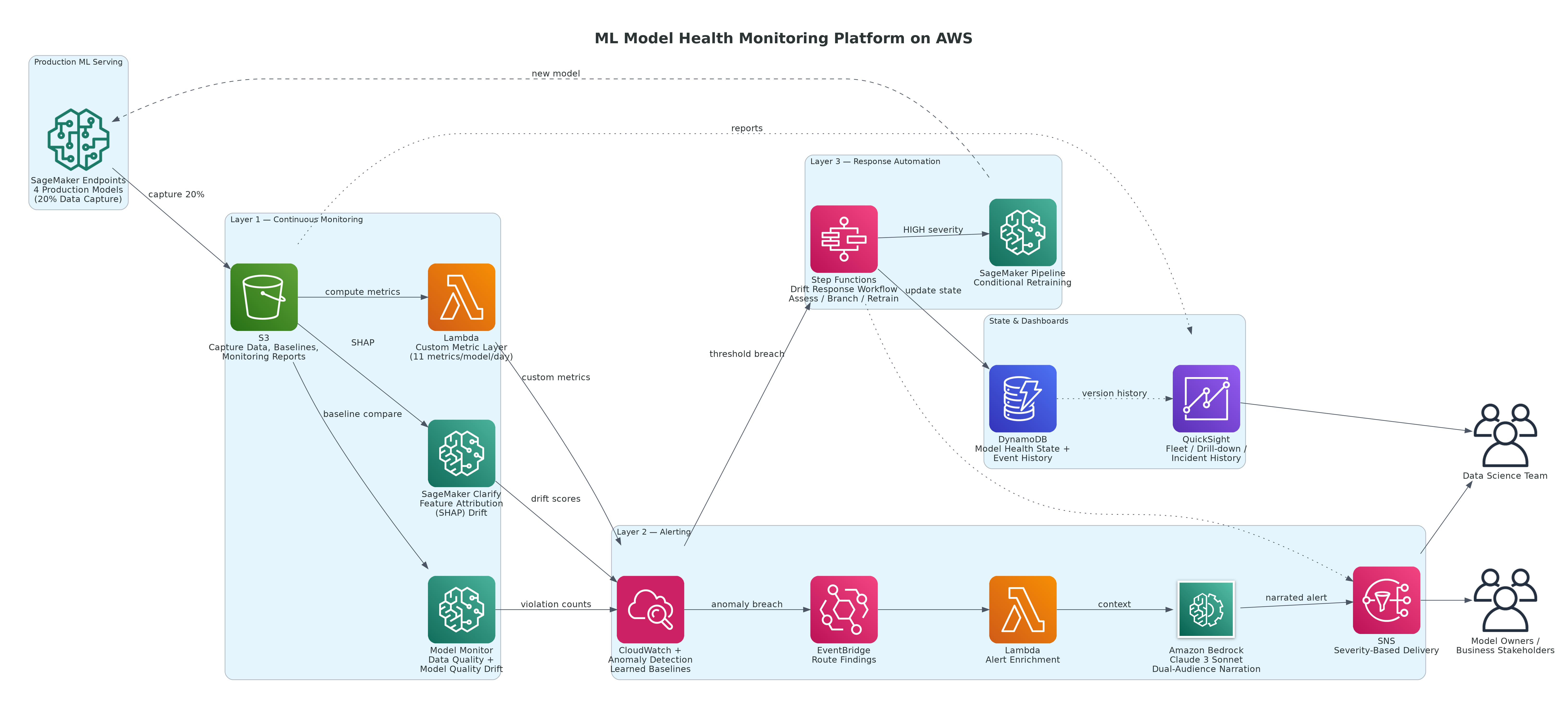
Figure 1: ML Model Health Monitoring Platform — Three-Layer Observability Architecture on AWS
AWS Services Used:
- Amazon SageMaker Model Monitor — automated data quality, model quality, feature attribution drift, and bias drift monitoring
- Amazon S3 — baseline statistics storage, monitoring reports, and model artifacts
- Amazon CloudWatch — custom metrics for prediction distribution, confidence score trends, and business-outcome correlation
- Amazon CloudWatch Anomaly Detection — ML-powered baseline for metric anomaly alerting
- Amazon EventBridge — routing Model Monitor findings to downstream alerting and response workflows
- AWS Lambda — custom metric computation, alert enrichment, and automated response triggers
- Amazon SNS — alert delivery to data science team, model owners, and business stakeholders
- Amazon QuickSight — model health dashboards with drill-down from fleet-level to individual feature level
- Amazon Bedrock (Claude 3 Sonnet) — natural language narration of drift findings for non-technical stakeholders
- Amazon DynamoDB — monitoring event history and model health state store
- AWS Step Functions — automated investigation and retraining trigger workflow
The architecture is organized into three layers: continuous monitoring that runs automatically against every production endpoint, alerting that routes findings to the right people at the right severity level, and response automation that initiates retraining when drift crosses defined thresholds.
Key Architectural Decisions
These are the decisions that shaped the monitoring platform — and the reasoning behind each one.
Decision 1: Why SageMaker Model Monitor Instead of Custom Monitoring Scripts?
When we began designing this platform, the data science team already had a collection of ad-hoc monitoring scripts — Python jobs that ran on a schedule, computed accuracy metrics against a sample of recent predictions, and emailed a CSV to a distribution list. The proposal to replace them with SageMaker Model Monitor initially met resistance: "We already have monitoring."
The gap was in what those scripts didn't catch. Custom accuracy scripts require ground truth labels — which for demand forecasting means waiting 30–90 days for actual sales data to come in before you can measure prediction accuracy. By the time the accuracy script fires an alert, the model has been making poor predictions for weeks.
SageMaker Model Monitor's data quality monitoring works on the input features themselves — no ground truth required. It detects when the distribution of inputs to the model has shifted away from the training baseline, which is an early warning signal for impending accuracy degradation, often days or weeks before accuracy metrics show it.
| Monitoring Type |
What It Catches |
Ground Truth Required |
Detection Lead Time |
| Custom accuracy scripts |
Accuracy drop after the fact |
Yes — often 30–90 day lag |
Days to weeks after degradation |
| SageMaker Data Quality Monitor |
Input feature distribution shift |
No |
Days before accuracy impact |
| SageMaker Model Quality Monitor |
Prediction accuracy vs. ground truth |
Yes |
When labels arrive |
| SageMaker Feature Attribution Drift |
SHAP value shifts across features |
No |
Days before accuracy impact |
| Custom CloudWatch metrics |
Business outcome correlation |
Partial |
Configurable |
The business decision: Data quality and feature attribution monitoring give you early warning before accuracy degrades. Accuracy monitoring tells you the model has already failed. For a business that makes decisions daily on model outputs, early warning is worth more than post-hoc confirmation.
Decision 2: Why Build a Custom Metric Layer on Top of Model Monitor?
SageMaker Model Monitor produces statistical monitoring reports — violations, constraint comparisons, distribution summaries. What it does not produce natively is business-aligned metrics: prediction confidence trend over the past 14 days, percentage of predictions in the high-confidence band vs. the uncertain band, correlation between model confidence and actual outcome accuracy, or the rolling 7-day prediction error by product category.
These are the metrics that business stakeholders can understand and act on. They are also the metrics that catch failure modes that statistical drift monitoring misses — specifically, cases where input distributions appear stable but the model's confidence is systematically shifting, which often precedes an accuracy drop on a specific segment of the data.
We built a Lambda-based custom metric layer that runs alongside Model Monitor, computing and publishing 11 custom CloudWatch metrics per model per day. CloudWatch Anomaly Detection then establishes a learned baseline for each metric and alerts when the metric deviates beyond the expected band.
The business decision: Statistical drift metrics are for data scientists. Business-outcome metrics are for the model owners who decide whether to retrain, adjust thresholds, or escalate. Both layers are necessary. Neither is sufficient alone.
Decision 3: Why Amazon Bedrock for Alert Narration?
A SageMaker Model Monitor violation report looks like this:
CODE
feature_name: units_sold_30d
constraint_check_type: distribution_statistics
description: Completeness check failed. Expected 0.98, Got 0.71
That output is actionable for a data scientist. It is not actionable for the demand planning manager who owns the model's business outcomes and needs to decide whether to hold a manual forecast review while the issue is investigated.
We added an Amazon Bedrock narration layer that converts Model Monitor violation reports and CloudWatch anomaly findings into plain-language summaries targeted at two audiences: a technical summary for the data science team and an executive summary for the model owner.
Example narration generated for a data quality violation on the demand forecasting model:
For the data science team: The units_sold_30d feature is showing 27% missing values in today's scoring batch, compared to a 2% baseline at training time. This is likely caused by a data pipeline upstream of the feature store — the feature relies on transaction data from the ERP integration, and the completeness drop coincides with the ERP maintenance window scheduled last night. Check the Glue ETL job for sales_transactions_daily before triggering retraining.
For the demand planning team: The demand forecasting model has detected an issue with one of its input data sources from last night. Today's predictions may be less reliable than usual for SKUs in the Electronics and Appliances categories. We recommend treating today's forecast output as indicative rather than definitive until the data science team confirms the issue is resolved — estimated by end of day.
That second paragraph is what prevents a business stakeholder from either ignoring a real issue or escalating a routine data pipeline hiccup into an emergency. It sets the right level of concern, in language that matches the audience, without requiring the data science team to write it manually for every alert.
The business decision: Monitoring without communication is incomplete. The alert needs to reach the right person with the right context and the right recommended action. Bedrock makes that possible at scale without manual effort.
Implementation Pattern
Setting Up SageMaker Model Monitor
Model Monitor requires three components per endpoint: a baseline computed from training data, a monitoring schedule that runs against live traffic, and a violation handler that routes findings downstream.
PYTHON
import boto3
import sagemaker
from sagemaker.model_monitor import (
    DefaultModelMonitor,
    DataCaptureConfig,
    CronExpressionGenerator
)
from sagemaker.model_monitor.dataset_format import DatasetFormat

sagemaker_session = sagemaker.Session()
role = sagemaker.get_execution_role()
bucket = "ml-monitoring-bucket"
endpoint_name = "demand-forecast-endpoint-prod"

# Step 1: Enable data capture on the endpoint
# This captures a sample of inference requests and responses to S3
data_capture_config = DataCaptureConfig(
    enable_capture=True,
    sampling_percentage=20,          # Capture 20% of traffic — sufficient for drift detection
    destination_s3_uri=f"s3://{bucket}/data-capture/{endpoint_name}",
    capture_options=["Input", "Output"],
    csv_content_types=["text/csv"],
    json_content_types=["application/json"]
)

# Apply to endpoint — update in place, no redeployment required
predictor = sagemaker.predictor.Predictor(
    endpoint_name=endpoint_name,
    sagemaker_session=sagemaker_session
)
predictor.update_data_capture_config(data_capture_config=data_capture_config)

# Step 2: Compute baseline statistics from training data
monitor = DefaultModelMonitor(
    role=role,
    instance_count=1,
    instance_type="ml.m5.xlarge",
    volume_size_in_gb=20,
    max_runtime_in_seconds=3600,
    sagemaker_session=sagemaker_session
)

monitor.suggest_baseline(
    baseline_dataset=f"s3://{bucket}/training-data/baseline.csv",
    dataset_format=DatasetFormat.csv(header=True),
    output_s3_uri=f"s3://{bucket}/baseline-results/{endpoint_name}",
    wait=True
)

# Step 3: Create daily monitoring schedule
monitor.create_monitoring_schedule(
    monitor_schedule_name=f"{endpoint_name}-data-quality-monitor",
    endpoint_input=endpoint_name,
    output_s3_uri=f"s3://{bucket}/monitoring-reports/{endpoint_name}",
    statistics=monitor.baseline_statistics(),
    constraints=monitor.suggested_constraints(),
    schedule_cron_expression=CronExpressionGenerator.daily(),
    enable_cloudwatch_metrics=True      # Publish violation counts to CloudWatch
)
Feature attribution drift monitoring runs in parallel using SageMaker Clarify, tracking SHAP value distributions across features to detect when the model's reliance on specific features has shifted — a subtler but often more informative signal than raw data distribution drift.
PYTHON
from sagemaker.clarify import (
    SageMakerClarifyProcessor,
    ModelConfig,
    ModelPredictedLabelConfig,
    SHAPConfig,
    DataConfig
)

clarify_processor = SageMakerClarifyProcessor(
    role=role,
    instance_count=1,
    instance_type="ml.m5.xlarge",
    sagemaker_session=sagemaker_session
)

shap_config = SHAPConfig(
    baseline=[
        # Baseline values for each feature — use training set means
        [2847, 0.73, 14.2, 3, 1, 0.91, 28, 0, 1, 0.84]
    ],
    num_samples=500,
    agg_method="mean_abs",
    save_local_shap_values=False
)

clarify_processor.run_explainability(
    data_config=DataConfig(
        s3_data_input_path=f"s3://{bucket}/data-capture/{endpoint_name}/recent/",
        s3_output_path=f"s3://{bucket}/explainability/{endpoint_name}",
        label="prediction",
        dataset_type="text/csv"
    ),
    model_config=ModelConfig(
        model_name="demand-forecast-model-v4",
        instance_type="ml.m5.xlarge",
        instance_count=1
    ),
    explainability_config=shap_config
)
Custom CloudWatch Metric Layer
The Lambda function runs daily after Model Monitor completes, pulling the captured inference data from S3, computing business-aligned metrics, and publishing them to CloudWatch under a custom namespace.
PYTHON
import boto3
import json
import numpy as np
from datetime import datetime, timedelta

s3 = boto3.client("s3")
cloudwatch = boto3.client("cloudwatch", region_name="ap-south-1")

def compute_and_publish_model_metrics(endpoint_name: str, bucket: str):
    """
    Compute business-aligned health metrics from captured inference data
    and publish to CloudWatch for anomaly detection and dashboarding.
    """
    # Load last 24 hours of captured inference data from S3
    prefix = f"data-capture/{endpoint_name}/{datetime.utcnow().strftime('%Y/%m/%d')}/"
    response = s3.list_objects_v2(Bucket=bucket, Prefix=prefix)

    predictions = []
    confidence_scores = []

    for obj in response.get("Contents", []):
        data = json.loads(
            s3.get_object(Bucket=bucket, Key=obj["Key"])["Body"].read()
        )
        for record in data.get("captureData", {}).get("endpointOutput", {}).get("data", []):
            pred = float(record.get("prediction", 0))
            conf = float(record.get("confidence", 0))
            predictions.append(pred)
            confidence_scores.append(conf)

    if not predictions:
        return

    metrics = [
        # % of predictions in high-confidence band (>0.80)
        {
            "MetricName": "HighConfidencePredictionRate",
            "Value": sum(1 for c in confidence_scores if c > 0.80) / len(confidence_scores),
            "Unit": "None"
        },
        # Mean confidence score — a downward trend precedes accuracy drops
        {
            "MetricName": "MeanPredictionConfidence",
            "Value": float(np.mean(confidence_scores)),
            "Unit": "None"
        },
        # Coefficient of variation — unusually high variance signals instability
        {
            "MetricName": "PredictionCoefficientOfVariation",
            "Value": float(np.std(predictions) / np.mean(predictions))
                     if np.mean(predictions) != 0 else 0,
            "Unit": "None"
        },
        # Predictions outside historical interquartile range — outlier rate
        {
            "MetricName": "OutOfRangePredictionRate",
            "Value": sum(
                1 for p in predictions
                if p < np.percentile(predictions, 5) or p > np.percentile(predictions, 95)
            ) / len(predictions),
            "Unit": "None"
        }
    ]

    cloudwatch.put_metric_data(
        Namespace=f"MLModelHealth/{endpoint_name}",
        MetricData=[
            {**m, "Timestamp": datetime.utcnow(), "Dimensions": [
                {"Name": "EndpointName", "Value": endpoint_name},
                {"Name": "Environment", "Value": "production"}
            ]}
            for m in metrics
        ]
    )
CloudWatch Anomaly Detection is then configured on each custom metric to establish a learned band based on 14 days of history. When a metric breaches the anomaly band, EventBridge routes the finding to the alert enrichment Lambda, which queries the monitoring history, assembles context, and calls Bedrock for narration before dispatching to SNS.
Bedrock Alert Narration
PYTHON
import boto3
import json

bedrock = boto3.client("bedrock-runtime", region_name="ap-south-1")

def narrate_drift_alert(alert_context: dict) -> dict:
    """
    Convert raw monitoring findings into plain-language summaries
    for two audiences: data science team and business model owner.
    """
    prompt = f"""You are an ML observability analyst. A production model health alert has been triggered.

Alert Details:
- Model: {alert_context['model_name']}
- Endpoint: {alert_context['endpoint_name']}
- Alert type: {alert_context['alert_type']}
- Triggered metric: {alert_context['metric_name']}
- Current value: {alert_context['current_value']}
- Expected range: {alert_context['expected_range']}
- Violation summary from SageMaker Model Monitor: {alert_context['violations']}
- Recent business context: {alert_context['business_context']}
- Model purpose: {alert_context['model_purpose']}

Write two summaries:

1. TECHNICAL SUMMARY (for the data science team): Explain what metric triggered, what it likely means technically, what to investigate first, and whether retraining is likely needed. Be specific.

2. BUSINESS SUMMARY (for the model owner): Explain in plain language what is happening, how it might affect decisions made using this model today, and what action they should take (if any) while the team investigates. Avoid technical jargon. Maximum 3 sentences.

Respond as a JSON object with keys: technical_summary (string), business_summary (string), recommended_action (string: one of INVESTIGATE, RETRAIN, ESCALATE, MONITOR)."""

    response = bedrock.invoke_model(
        modelId="anthropic.claude-3-sonnet-20240229-v1:0",
        contentType="application/json",
        accept="application/json",
        body=json.dumps({
            "anthropic_version": "bedrock-2023-05-31",
            "max_tokens": 600,
            "temperature": 0.1,     # Very low temperature — consistent, factual narration
            "messages": [{"role": "user", "content": prompt}]
        })
    )

    result = json.loads(response["body"].read())
    return json.loads(result["content"][0]["text"])
Automated Response: Step Functions Retraining Workflow
When drift severity crosses a defined threshold — specifically, when data quality violations exceed 15% of monitored features or feature attribution drift exceeds 0.25 on any top-5 SHAP feature — Step Functions triggers an automated investigation and conditional retraining workflow.
CODE
CloudWatch Alarm (drift threshold breached)
    → EventBridge rule
    → Step Functions: ModelDriftResponseWorkflow
        → State 1: AssessViolationSeverity
              Query Model Monitor reports from last 3 days
              Compute trend: is drift accelerating or stable?
        → State 2 (branch on severity):
              LOW: Publish enhanced monitoring alert, increase
                   capture sampling to 50%, notify data science team
              MEDIUM: Trigger data validation job on feature store,
                      notify model owner + data science team,
                      schedule retraining review in 48 hours
              HIGH: Trigger SageMaker Pipeline retraining immediately,
                    notify all stakeholders, flag predictions
                    as "under review" in the serving layer
        → State 3: UpdateModelHealthState (DynamoDB)
        → State 4: NotifyStakeholders (SNS → Bedrock narration)
This workflow means that a high-severity drift event triggers an automatic retraining run without requiring a data scientist to manually initiate it at 2am — while still routing appropriate notifications so the team can validate the retrained model before it goes live.
QuickSight Model Health Dashboard
The QuickSight dashboard consumes data from three sources: Model Monitor reports stored in S3, custom CloudWatch metrics exported via a Lambda-based ETL to S3, and model version history stored in DynamoDB. It is organized in three views:
- Fleet view: All four production models at a glance, with a RAG (Red/Amber/Green) health status for each based on composite drift score. The first screen any data science team member sees in the morning.
- Model drill-down: Per-model view showing data quality violation trend (30 days), feature attribution drift per feature (heatmap), confidence score trend, and prediction distribution vs. training baseline.
- Incident history: Timeline of all drift alerts, the Bedrock-generated narratives, actions taken, and time-to-resolution — building the audit trail that compliance and leadership need.
Cost Architecture and AWS Service Spend
At steady-state monitoring four production SageMaker endpoints with daily monitoring schedules:
| Service |
Usage |
Estimated Monthly Cost |
| SageMaker Model Monitor |
4 endpoints × daily schedule, ml.m5.xlarge processing |
~$96 |
| SageMaker Clarify (SHAP drift) |
4 runs/week × ml.m5.xlarge |
~$58 |
| Amazon S3 |
~180 GB (capture data, reports, baselines) |
~$4 |
| Amazon CloudWatch |
44 custom metrics, anomaly detection on 16 metrics, 120 alarms |
~$38 |
| AWS Lambda |
~180K invocations/month (metric computation + alert enrichment) |
~$2 |
| Amazon Bedrock (Claude 3 Sonnet) |
~60 narration calls/month (alert events only) |
~$1 |
| AWS Step Functions |
~12 workflow executions/month |
~$1 |
| Amazon SNS |
~200 alert notifications/month |
~$1 |
| Amazon QuickSight |
3 authors, 8 readers |
~$54 |
| Amazon DynamoDB |
Monitoring state store, low volume |
~$3 |
| Total |
|
~$258/month |
The cost profile is dominated by SageMaker processing instances running the monitoring jobs. The Bedrock narration cost is negligible — approximately $1/month for the volume of alerts a healthy production ML platform generates — because Bedrock is only invoked when a real alert fires, not on every monitoring run.
Against the cost of one silent drift incident — the retail client's demand forecasting drift resulted in an estimated ₹28–34 lakh in suboptimal inventory positioning over the 11 weeks it went undetected — the monitoring platform's infrastructure cost is recovered in the first incident it prevents.
Common Pitfalls (Real Lessons)
| Pitfall |
What Happened |
How We Fixed It |
| Baseline computed on a small training sample |
Model Monitor flagged 60% of features as drifted on day one — all false positives |
Recomputed baseline on full training dataset; minimum 10,000 records required |
| Alert thresholds set too tight on high-variance features |
PagerDuty fatigue — team started ignoring alerts within two weeks |
Analyzed 30-day metric history before setting thresholds; applied percentile-based bands not fixed values |
| Data capture at 100% sampling |
S3 storage costs ballooned to $340/month in week one |
Set sampling to 20% — statistically sufficient for drift detection at our volumes |
| Step Functions retraining triggered on a data pipeline outage |
Model retrained on 3 days of incomplete data, performance regressed |
Added data completeness gate before retraining trigger: >95% feature completeness required |
| QuickSight dashboard showed raw violation counts |
Business stakeholders interpreted every violation as a crisis |
Changed primary metric to composite health score (0–100) with clear RAG thresholds and plain-language status descriptions |
Each of these mistakes was instructive. The hardest lesson was the alert threshold problem — a monitoring system that people stop reading is worse than no monitoring at all, because it creates a false sense of coverage while providing none.
Business Outcomes
| Metric |
Before |
After |
Business Impact |
| Mean time to detect model degradation |
~47 days |
< 72 hours |
Drift caught before business decisions are affected |
| Monitoring coverage |
1 of 4 models (ad hoc) |
4 of 4 models (automated, continuous) |
Full production fleet visibility |
| Data science time on reactive investigation |
~35% of sprint capacity |
~8% of sprint capacity |
Freed for model improvement work |
| Silent drift incidents (annualised) |
3 known, unknown unknowns |
0 since platform launch |
Planning team trust in model outputs restored |
| Stakeholder alert actionability |
Raw violation reports — ignored |
Bedrock-narrated, audience-targeted alerts |
Right action taken within 4 hours of alert |
| Compliance audit readiness |
No documentation trail |
Full incident history with actions and resolutions |
Audit-ready model governance record |
The most significant shift was not technical — it was cultural. Before the monitoring platform, the data science team was in a reactive posture: something would break, someone would complain, the team would investigate. After the platform, the team is in a proactive posture: the system alerts them to an emerging issue, they investigate and resolve it before it surfaces as a business complaint. That shift from reactive to proactive is the organizational value of model observability, and it doesn't appear on an AWS cost report.
Lessons for Technology Leaders
- A model that produces predictions without health visibility is a liability, not an asset — Every ML model in production is making a claim about the world. As the world changes, that claim becomes less reliable. Without continuous monitoring, you have no way to know when to stop trusting it — and neither does the business.
- Data quality monitoring is more valuable than accuracy monitoring for models with delayed ground truth — If your model's outcomes take weeks or months to observe, waiting for accuracy metrics means waiting for the damage to be done. Monitor the inputs. Input distribution shift is an early warning signal for accuracy degradation — often days or weeks ahead of the accuracy drop itself.
- Monitoring thresholds must be calibrated on real traffic, not set by intuition — Thresholds set too tight create alert fatigue and teams that ignore monitoring. Thresholds set too loose miss real issues. Spend the time analyzing 30 days of metric history before setting any threshold. The time investment pays back in monitoring that people actually trust and act on.
- Alert communication is a product, not a side effect — An alert that a data scientist understands but a business stakeholder ignores is a monitoring failure. Invest in audience-targeted communication. The Bedrock narration layer added minimal cost and dramatically changed how quickly appropriate actions were taken on drift events.
- Automated response is the destination, not the starting point — Start with alerting. Add dashboards. Build stakeholder trust in the monitoring data. Only then introduce automated retraining triggers — once the team has validated that the monitoring signals are reliable enough to act on autonomously. Automation built on unvalidated signals creates more problems than it solves.
About the Author
Chandni Gadhvi is Program Manager – Data and AI at AeonX Digital Technology Limited, where she leads the architecture and delivery of cloud-native AI and MLOps solutions for enterprise customers. She specializes in building production-grade ML systems on AWS that are observable, governable, and continuously improving. She is an advocate for operationally mature AI — the kind that earns and keeps business trust over time — and shares technical thought leadership to help engineering teams close the gap between ML in development and ML in production.
by Rajat Jindal | Apr 23, 2026 | AWS
The Pipeline Problem Nobody Talks About in Board Meetings
Every enterprise I work with has the same invisible cost centre: ETL pipelines. Hundreds of them. Running nightly. Breaking silently. Consuming 30-40% of data engineering capacity not to create value, but to move data from where it is to where it needs to be.
ETL — Extract, Transform, Load — was a necessary evil in a world where operational databases and analytics systems were architecturally incompatible. You could not run an analytical query against your production MySQL database without degrading customer-facing performance. So you moved the data. Every night. Through fragile, hand-coded pipelines that nobody fully understood and everybody feared changing.
In 2026, this model is not just expensive — it is architecturally incompatible with AI. AI agents need fresh data. Embedding pipelines need real-time updates. Knowledge Bases need to reflect the current state of your business, not last night’s snapshot. Every hour of ETL latency is an hour where your AI is answering questions with stale information — and stale AI answers erode user trust faster than no AI at all.
AWS Zero-ETL integrations eliminate this entire layer. Not by building better pipelines — by eliminating the need for pipelines altogether. Data flows continuously from operational sources to analytics and AI destinations without any pipeline code, scheduling infrastructure, or failure-mode complexity.
This post is about the strategic implications of that shift — and why the enterprises that adopt Zero-ETL first will free 30-40% of their data engineering capacity for AI innovation instead of pipeline maintenance.
Why ETL Pipelines Are the Silent Tax on Every AI Initiative
The Hidden Cost
In every data & AI presales discovery I run, I ask the same question: “What percentage of your data engineering team’s time is spent building and maintaining data movement pipelines versus building AI features or analytical capabilities?”
The answer, consistently, across industries: 30-50%. Sometimes higher.
That is not engineering time spent creating business value. It is engineering time spent ensuring that data arrives at the right place, in the right format, at the right time — work that has zero business differentiation. Every enterprise runs similar pipelines. None of them gain competitive advantage from having better COPY commands.
The Freshness Problem
ETL pipelines run on schedules — typically nightly. That means:
- Your analytics dashboard shows yesterday’s state, not today’s
- Your AI agent answers questions based on data that is 8-24 hours stale
- Your embedding pipeline generates vectors from last night’s snapshot, missing today’s customer interactions entirely
For traditional BI, nightly freshness was acceptable. For AI systems that users interact with in real-time, it creates a trust problem. When an employee asks “What is this customer’s current status?” and the AI answers based on yesterday’s data, that employee stops trusting the AI after the second incorrect answer.
The Fragility Problem
Every ETL pipeline is a potential failure point:
- Schema changes in the source database break the pipeline silently
- Network issues between source and destination create data gaps that go undetected for days
- Resource contention during peak ETL windows slows both the pipeline and production workloads
- A single failed dependency in a pipeline DAG can cascade and delay the entire data platform
The operations overhead of monitoring, alerting, retrying, and debugging ETL failures is substantial — and it scales linearly with the number of pipelines. More data sources = more pipelines = more fragility = more engineering time spent on maintenance.
What Zero-ETL Actually Means: A Technical and Strategic Definition
Zero-ETL is not “better ETL.” It is the architectural elimination of the pipeline layer entirely.
With Zero-ETL integrations, data replicates continuously from the operational source to the analytics or AI destination using native AWS infrastructure. There is no pipeline code to write. No scheduler to configure. No failure modes to handle. No transformation jobs to maintain.
How It Works (Architecturally)
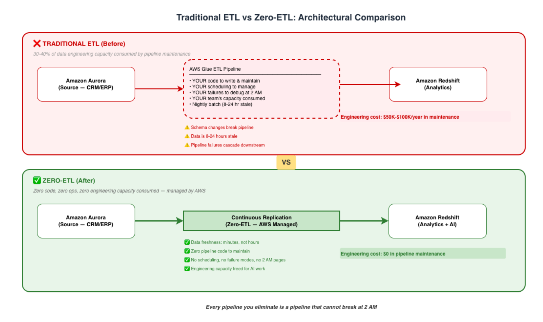
Available Zero-ETL Integrations on AWS (as of early 2026)
| Source |
Destination |
Use Case |
| Amazon Aurora MySQL |
Amazon Redshift |
Operational data → analytics without pipelines |
| Amazon Aurora PostgreSQL |
Amazon Redshift |
Same — for PostgreSQL workloads |
| Amazon RDS for MySQL |
Amazon Redshift |
Non-Aurora RDS → analytics |
| Amazon DynamoDB |
Amazon Redshift |
NoSQL operational data → SQL analytics |
| Amazon DynamoDB |
Amazon OpenSearch |
NoSQL data → search and vector search |
| Amazon Aurora |
Amazon OpenSearch |
Relational data → search (including semantic) |
The Strategic Implication
Every integration in that table eliminates one or more ETL pipelines — plus the scheduling, monitoring, alerting, and debugging infrastructure around them. For a mid-market enterprise with 20-50 ETL pipelines, Zero-ETL can eliminate 30-60% of them within a single quarter.
The AI Angle: Why Zero-ETL Is an AI Enablement Strategy
Zero-ETL is typically discussed as an analytics optimisation. That undersells it dramatically. For enterprises deploying AI, Zero-ETL is a freshness and velocity strategy that directly impacts AI quality.
Freshness Enables AI Trust
When Aurora transactional data flows continuously to Redshift (and from there to Bedrock Knowledge Bases), your AI is always grounded in current state. The customer who placed an order 10 minutes ago appears in the AI’s answers immediately — not tomorrow morning after the nightly batch runs.
This matters enormously for:
- Customer-facing AI: “What’s the status of my order?” must reflect the current state
- Internal copilots: “What’s our pipeline this quarter?” must include today’s deals
- AI agents: Autonomous agents making decisions on stale data make wrong decisions
Velocity Enables AI Experimentation
The most expensive property of AI development is iteration speed. When every new AI use case requires a new ETL pipeline to get data into the right format and place, the cycle time for each experiment is weeks. When data is already available in Redshift and OpenSearch via Zero-ETL, a new AI use case requires only a Bedrock Knowledge Base configuration — deployable in hours.
Example: CRM Data Flowing to AI Without Pipelines
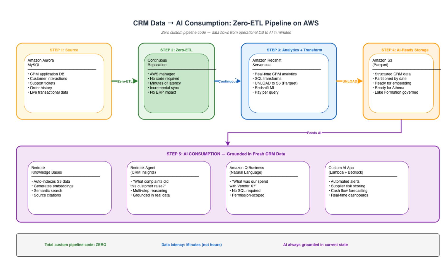
In this pattern, CRM data flows from Aurora to Redshift via Zero-ETL (zero code), then from Redshift to S3 via scheduled UNLOAD (one command), then into Bedrock Knowledge Bases for AI consumption. Total custom pipeline code: zero. Total latency: minutes, not hours.
Implementation: Setting Up Zero-ETL (Aurora → Redshift)
# Create a Zero-ETL integration from Aurora MySQL to Redshift
aws rds create-integration \
  --integration-name crm-zero-etl \
  --source-arn arn:aws:rds:ap-south-1:<account-id>:cluster:crm-aurora-cluster \
  --target-arn arn:aws:redshift-serverless:ap-south-1:<account-id>:namespace/<namespace-id> \
  --tags Key=Environment,Value=Production Key=Purpose,Value=AI-Analytics
Step 2: Authorise the Integration on Redshift
-- Run in Redshift: create the database from the integration
CREATE DATABASE crm_realtime FROM INTEGRATION '<integration-id>';

-- Data is now continuously available — query it immediately
SELECT customer_id, interaction_type, created_at
FROM crm_realtime.public.customer_interactions
WHERE created_at > CURRENT_DATE - INTERVAL '1 hour';
Step 3: Feed AI From Redshift
-- Unload fresh CRM data to S3 for Bedrock Knowledge Base consumption
UNLOAD ('
  SELECT customer_id, subject, body, resolution_status, created_at
  FROM crm_realtime.public.customer_interactions
  WHERE created_at > CURRENT_DATE - INTERVAL ''1 day''
')
TO 's3://data-lake-ai-ready/crm/daily/'
IAM_ROLE 'arn:aws:iam::<account-id>:role/RedshiftUnloadRole'
FORMAT PARQUET
ALLOWOVERWRITE;
This three-step pattern — Zero-ETL into Redshift, UNLOAD to S3, Bedrock Knowledge Base on S3 — gives you a continuously fresh AI data pipeline with zero custom ETL code.
The Business Case: Pipeline Elimination Economics
What You Stop Paying For
| Eliminated Cost |
Annual Savings (Mid-Market) |
Notes |
| Glue job compute (nightly batch ETL) |
$15K-$40K/year |
Depends on data volume and job complexity |
| Data engineer pipeline maintenance (30-40% of time) |
$50K-$100K/year |
1-2 FTE equivalent redirected to AI work |
| Incident response for pipeline failures |
$15K-$30K/year |
On-call time, investigation, remediation |
| Data freshness penalty (stale dashboards, stale AI) |
Unquantified but material |
Decisions made on old data have compounding cost |
| Total pipeline elimination value |
$80K-$170K/year |
— |
What You Start Paying For
| Zero-ETL Cost |
Annual Cost |
Notes |
| Zero-ETL integration (Aurora → Redshift) |
Included in Redshift pricing |
No separate charge for the integration itself |
| Redshift Serverless compute |
$30K-$80K/year |
Usage-based — pay for what you query |
| Net savings |
$15K-$130K/year |
Plus engineering capacity freed for AI |
The real ROI is not the infrastructure savings — it is the engineering capacity. Every data engineer freed from pipeline maintenance is a data engineer who can build AI features, train models, or optimise data quality. That reallocation is what accelerates AI adoption.
A Presales Perspective: Positioning Zero-ETL in Customer Conversations
The Question That Opens the Conversation
“How many ETL pipelines does your data team maintain today? And how many of them broke in the last 30 days?”
The first number is usually 20-100. The second number makes the room uncomfortable. That discomfort is the opening.
The Framing That Resonates
For CTOs: “Every pipeline is technical debt that consumes engineering capacity you could be spending on AI. Zero-ETL eliminates that debt category-by-category.”
For CDOs: “Your data freshness SLA is limited by your slowest pipeline. Zero-ETL makes freshness an infrastructure property, not an engineering challenge.”
For CFOs: “You are paying senior data engineers $150K-$200K to maintain COPY commands that AWS will run for you at infrastructure cost. That is a misallocation of your most expensive resource.”
The Objection You Will Hear
“We have custom transformations in our ETL — Zero-ETL can’t replace those.”
Response: “Correct. Zero-ETL replaces the data movement layer — the extract and load. Your custom transformation logic moves to Redshift (SQL transforms, Redshift ML) or to downstream processing. The transformation is still yours — you just stop paying for the plumbing around it.”
Not every pipeline disappears. But the 40-60% that are pure data movement with minimal transformation — those are immediately eliminable. Start there.
When to Use Zero-ETL vs Traditional Approaches
| Scenario |
Recommendation |
Why |
| Aurora/RDS data needed in Redshift for analytics + AI |
Zero-ETL |
Eliminates pipeline entirely |
| DynamoDB data needed for search/AI |
Zero-ETL to OpenSearch |
Enables vector search without ETL |
| Complex multi-source joins and transformations |
Glue ETL (keep) |
Transformation logic still needs code |
| Real-time streaming from external sources |
Kinesis + Glue Streaming |
Zero-ETL is for AWS-to-AWS sources |
| One-time historical data migration |
AWS DMS |
Zero-ETL is for ongoing replication |
Zero-ETL does not replace all pipelines. It replaces the ones that should never have been pipelines in the first place — pure data replication between AWS services that historically required engineering effort for no differentiated value.
The 12-Month Roadmap: From Pipeline-Heavy to Zero-ETL
| Month |
Action |
Outcome |
| 1 |
Audit existing pipelines — categorise as “pure movement” vs “transformation” |
Know which pipelines are eliminable |
| 2-3 |
Enable Zero-ETL for primary Aurora → Redshift flows |
3-5 pipelines eliminated, data freshness improved to minutes |
| 4-5 |
Migrate DynamoDB → OpenSearch pipelines to Zero-ETL |
Search and vector search fed automatically |
| 6-8 |
Connect Redshift to Bedrock Knowledge Bases via S3 UNLOAD |
AI consumption without custom integration |
| 9-12 |
Redeploy freed engineering capacity to AI use cases |
Data engineers building AI features, not maintaining pipes |
Lessons for Technology Leaders
- Every pipeline you eliminate is a pipeline that cannot break at 2 AM — Reliability is not about building better monitoring for your pipelines. It is about having fewer pipelines to monitor.
- Zero-ETL is a capacity strategy, not just a cost strategy — The $15K-$40K in Glue savings matters less than the $60K-$120K in engineering time redirected from maintenance to AI innovation.
- Data freshness is an AI quality metric — When your AI answers questions based on yesterday’s data, users stop trusting it. Zero-ETL’s continuous replication keeps AI grounded in current state.
- Not every pipeline should be Zero-ETL — Complex multi-source transformations still need Glue or custom code. But pure data replication (40-60% of most enterprise pipelines) should never be custom code. Eliminate those first.
- The CTO who says “our pipelines work fine” has not asked their data engineers how they feel about it — Pipelines “working” and pipelines being a good use of expensive engineering talent are different statements. Ask the team — they will tell you where the waste is.
About the Author
Rajat Jindal is VP – Presales at AeonX Digital Technology Limited, where he architects winning cloud strategies for enterprise customers and translates modernization into measurable business value. He is a strong advocate of AWS, committed to sharing thought leadership that helps technology leaders make faster, better-informed decisions.
by Chandni Gadhvi | Apr 15, 2026 | AWS
The Quality Intelligence Imperative: Why Manual Inspection Is a Manufacturing Risk
In high-volume manufacturing, quality inspection is one of the last processes to be digitally transformed — and often one of the most expensive when it isn't.
The reason manual inspection persists is understandable: it feels controllable. You can see the inspectors working, count the headcount, measure attendance. What you cannot easily measure is the inspection you missed on the 200th unit at the end of a shift, the subtle assembly defect that gets through because two inspectors interpreted the standard differently, or the batch-level failure that could have been caught at the individual unit level if your data had been structured enough to see the pattern forming.
When we engaged with an automotive component manufacturer facing these challenges, the gap between their inspection model and their quality outcomes was measurable and expensive: 82% inspection accuracy with 100% manual coverage, a defect escape rate that was generating warranty claims and OEM escalations, and no digital record of what had been inspected, when, or by whom.
The problem wasn't effort — the inspection team was working. The problem was that manual inspection at production speed is physiologically limited. Human attention degrades with volume, lighting variation, shift fatigue, and cognitive load. AI does not have those constraints.
This post documents how we designed and deployed a real-time AI-powered visual inspection platform for that manufacturer — combining YOLOv11 edge inference with Amazon Bedrock's generative intelligence and AWS IoT-based cloud ingestion to deliver what manual inspection could not: consistent, traceable, continuously improving quality coverage at full production speed.
As Technical Architect for this initiative at AeonX Digital, I led the architecture design, model strategy, and AWS service selection across the edge and cloud layers. What follows covers the implementation in enough detail to be useful to practitioners, along with the architectural decisions and trade-offs that shaped each choice.
The outcome: inspection accuracy increased from 82% to 97%, quality-related costs reduced by approximately 35% annually, and the manufacturer moved from sample-based inspection to full AI-driven coverage on every unit produced.
Why This Matters Now: The Edge AI Inflection Point in Manufacturing
Three forces are converging to make AI-powered inspection a mainstream manufacturing capability rather than a pilot project:
- Edge compute has reached production-grade reliability — NVIDIA Jetson AGX Orin and similar edge AI platforms now deliver inference speeds that match assembly line cycle times. The latency barrier that made cloud-only AI inspection impractical is gone. Inference happens at the device, in single-digit milliseconds, with no dependency on network connectivity for the primary quality decision.
- Computer vision models have matured for industrial use — Transfer learning from large pretrained models like YOLO architectures means that a manufacturer no longer needs tens of thousands of defect images to build a high-accuracy detector. Fine-tuning on a few thousand labeled images now produces production-grade accuracy in days, not months.
- Generative AI closes the gap between detection and action — Traditional computer vision tells you what it found. It doesn't tell you what to do about it. Amazon Bedrock converts detection outputs into plain-language summaries, corrective action recommendations, and trend narratives that a plant supervisor can act on without interpreting bounding boxes and confidence scores.
The decision to build this system was driven by a quality leadership team that recognized manual inspection was no longer scaling with production volume — and that the cost of escaped defects had begun to exceed the cost of building a better system.
The Business Problem
The manufacturer's existing inspection workflow had:
- 100% manual inspection with no structured defect criteria — consistent judgment depended entirely on individual inspector experience
- No real-time alerting — defect patterns were visible only in end-of-shift reports, after hundreds of units had already been produced
- No digital audit trail per unit — traceability for OEM compliance was manual and incomplete
- No predictive capability — root cause analysis happened after warranty claims, not before
- Sample-based documentation — only a fraction of inspected units had any recorded evidence
Business impact of the status quo:
- Rising rework costs from defects caught late in the production process
- OEM escalations and warranty claims from defects caught by customers
- Inability to scale inspection headcount proportionally with production volume increases
- Compliance exposure from incomplete traceability records
The goal was not to assist manual inspection — it was to replace it with a system that was faster, more consistent, and fully traceable, while keeping quality engineers in the loop as analysts rather than inspectors.
Technical Architecture: Edge + Cloud + GenAI
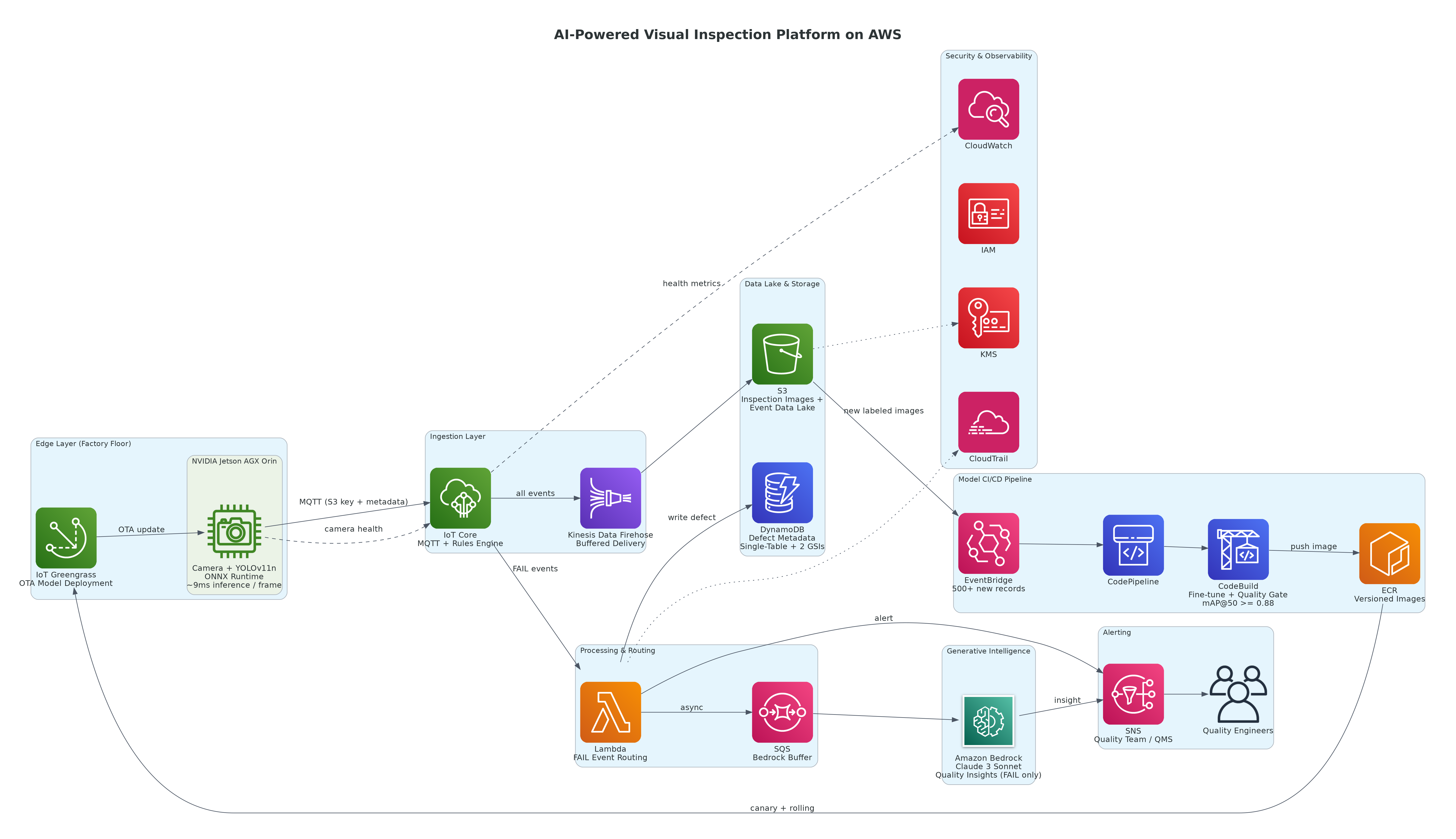
Figure 1: AI-Powered Visual Inspection Platform — Edge + Cloud + GenAI Reference Architecture
AWS and Technology Stack:
- YOLOv11n (Ultralytics) — custom-trained object detection models on NVIDIA Jetson AGX Orin edge devices
- ONNX Runtime — edge inference engine for runtime-agnostic deployment
- AWS IoT Core — secure MQTT ingestion from edge to cloud
- Amazon Kinesis Data Firehose — buffered delivery to S3 data lake
- Amazon S3 — inspection image and event data lake
- Amazon DynamoDB — structured defect metadata with single-table design
- Amazon Bedrock (Claude 3 Sonnet) — generative quality insights for FAIL events
- Amazon SNS — real-time alerting to quality teams and QMS
- AWS IoT Greengrass — OTA model deployment to edge devices
- AWS CodePipeline + Amazon ECR — automated model retraining and deployment pipeline
- Amazon CloudWatch and CloudTrail — observability and compliance audit
- AWS KMS and IAM — encryption and access control
The architecture combines three layers: edge inference for latency-critical pass/fail decisions, cloud data lake for analytics and model retraining, and generative AI for converting detections into actionable insights. Each layer was designed to be independently scalable and replaceable.
Key Architectural Decisions
Decision 1: Why Edge Inference Instead of Cloud Inference?
The first architectural question for any computer vision deployment in manufacturing is where inference runs. Cloud inference is simpler to operate — you push images to an API and get results back. The problem is latency.
At five units per minute on an assembly line, the maximum acceptable inspection-to-decision time is 180ms. A round-trip cloud API call — accounting for image upload, inference, and response — consistently exceeds 300–400ms under normal network conditions, and is completely unavailable during network interruptions.
Edge inference on NVIDIA Jetson AGX Orin with ONNX Runtime delivers 9ms per frame. That is not incremental improvement over cloud inference — it is a fundamentally different latency class that makes real-time line-speed inspection possible.
| Approach |
Inference Latency |
Network Dependency |
Cost at Scale |
| Cloud inference (API) |
300–400ms |
Hard dependency |
High — every frame billed |
| Edge inference (ONNX) |
~9ms |
None for primary decision |
Low — compute is local |
| Edge inference (TensorRT FP16) |
~4.5ms |
None |
Low — optimized for device |
The business decision: Production lines do not pause for network issues. Edge inference removes the network from the critical path for the primary quality decision. Cloud connectivity is required for analytics, alerting, and model updates — but not for the inspection itself.
Decision 2: Why YOLOv11n Over Larger Model Variants?
We benchmarked three YOLOv11 variants during model selection:
- YOLOv11n (nano): mAP@50 of 0.91 after fine-tuning, 9ms inference latency on Jetson AGX Orin
- YOLOv11s (small): mAP@50 of 0.94, 21ms inference latency
- YOLOv11m (medium): mAP@50 of 0.96, 38ms inference latency
The 3–5 percentage point accuracy improvement from larger models was real but insufficient to justify the latency trade-off. At 5 units per minute, 21ms is already marginal headroom. At 38ms, the model cannot keep pace with line speed at all production rates. YOLOv11n at 9ms gives 20× headroom over cycle time — sufficient buffer for device temperature variation, I/O overhead, and future production rate increases.
The business decision: Accuracy matters, but availability matters more. A model with 91% mAP that runs reliably at every production rate is more valuable than a 96% mAP model that creates line stoppages during rate increases.
The defect metadata workload is write-intensive: at 72,000 inspections per day across three production lines, the system generates sustained write throughput with short burst peaks during production starts and end-of-line inspections.
We evaluated Aurora PostgreSQL first, given the team's familiarity with SQL. The decision shifted to DynamoDB for three specific reasons:
- Burst write handling without connection pooling — RDS connection pools become a bottleneck under burst write conditions. DynamoDB on-demand capacity handles burst transparently without connection management overhead.
- Access patterns were well-defined — The three primary query patterns (by product unit, by station + time range, by shift + defect class) mapped cleanly to a single-table design with two GSIs. No ad-hoc joins were required.
- TTL-based retention — Compliance required one-year defect record retention followed by automatic deletion. DynamoDB's native TTL feature handles this without a separate archival job.
The business decision: DynamoDB's operational simplicity at the write volumes this workload generates outweighed Aurora's query flexibility for access patterns that are well-understood in advance.
Implementation Pattern
YOLOv11 Model Training: Dataset and Configuration
Model training was the most labor-intensive phase of the project. The dataset comprised 11,400 labeled images across six defect classes: missing fastener, misaligned bracket, incorrect cable routing, surface scratch, incomplete weld, and foreign object presence. Annotation was performed in CVAT with double-blind review by quality engineers to ensure label consistency across inspectors.
PYTHON
from ultralytics import YOLO

# Fine-tune YOLOv11n on defect dataset
model = YOLO("yolo11n.pt")  # COCO-pretrained base weights

results = model.train(
    data="defect_dataset.yaml",    # Class names, train/val/test paths
    epochs=100,
    imgsz=640,
    batch=16,
    device="cuda:0",               # NVIDIA Jetson AGX Orin (2048 CUDA cores)
    optimizer="AdamW",
    lr0=0.001,
    lrf=0.01,
    momentum=0.937,
    weight_decay=0.0005,
    augment=True,
    patience=15,                   # Early stopping — critical for small defect classes
    cos_lr=True,                   # Cosine LR decay — more stable fine-tuning
    project="quality_inspection",
    name="yolov11_defect_v3",
    save=True,
    val=True
)

# Export to ONNX for runtime-agnostic edge deployment
model.export(format="onnx", dynamic=True, simplify=True)
Model performance after fine-tuning:
| Metric |
COCO Pretrained Only |
Fine-tuned v3 |
| mAP@50 |
0.58 |
0.91 |
| mAP@50-95 |
0.39 |
0.77 |
| Precision |
0.71 |
0.93 |
| Recall |
0.65 |
0.90 |
| Inference latency (Jetson AGX Orin, ONNX) |
~6ms |
~9ms |
Data augmentation — horizontal flip, brightness jitter (±20%), random rotation (±5°), and mosaic augmentation — was essential for handling ambient lighting variation across three production shifts. Without augmentation, the model performed well under optimal lighting and poorly in early morning conditions when production lighting takes time to stabilize.
Secure IoT Ingestion: MQTT Topic Design
CODE
manufacturing/{plant_id}/line/{line_id}/station/{station_id}/inspection
manufacturing/{plant_id}/line/{line_id}/station/{station_id}/camera/health
manufacturing/{plant_id}/alerts/defects
Each inspection event published to IoT Core:
JSON
{
  "event_id": "insp-20241118-STN12-04231",
  "timestamp": "2024-11-18T08:43:17.823Z",
  "plant_id": "PLANT-MH-01",
  "line_id": "LINE-03",
  "station_id": "STN-12",
  "product_id": "PROD-VAR-B-00892",
  "inspection_result": "FAIL",
  "defects": [
    {
      "class": "missing_fastener",
      "confidence": 0.91,
      "bounding_box": [412, 318, 56, 48]
    }
  ],
  "model_version": "yolov11_defect_v3",
  "inference_latency_ms": 9,
  "image_s3_key": "inspections/2024/11/18/LINE-03/STN-12/insp-04231.jpg"
}
IoT device policies enforced least-privilege — each edge device could publish only to its own station topic hierarchy, preventing cross-station data injection. IoT Core rules engine routed all events to Kinesis Data Firehose for S3 delivery, FAIL events additionally to Lambda for DynamoDB write and SNS alert, and camera health events to CloudWatch metrics.
DynamoDB Single-Table Design
PYTHON
import boto3
from datetime import datetime

dynamodb = boto3.resource("dynamodb", region_name="ap-south-1")
table = dynamodb.Table("QualityInspectionEvents")

def record_defect(event: dict):
    table.put_item(
        Item={
            # PK/SK: lookup by product unit for traceability report
            "PK": f"PRODUCT#{event['product_id']}",
            "SK": f"INSPECTION#{event['timestamp']}",

            # GSI-1: station + time range for root cause analysis
            "GSI1PK": f"STATION#{event['station_id']}",
            "GSI1SK": event["timestamp"],

            # GSI-2: shift + defect class for quality dashboard aggregation
            "GSI2PK": f"SHIFT#{event['shift_id']}",
            "GSI2SK": f"CLASS#{event['defects'][0]['class']}",

            "inspection_result": event["inspection_result"],
            "defects": event["defects"],
            "model_version": event["model_version"],
            "image_s3_key": event["image_s3_key"],
            "plant_id": event["plant_id"],
            "line_id": event["line_id"],
            "ttl": int(datetime.now().timestamp()) + (365 * 24 * 3600)
        }
    )
Generative AI Interpretation: Bedrock on FAIL Events Only
Traditional computer vision tells plant supervisors what was detected. Amazon Bedrock tells them what to do about it.
We integrated Bedrock only for FAIL inspection events — approximately 14% of total volume. This keeps Bedrock spend proportional to business value: a PASS result requires no natural language explanation.
Example: a missing fastener detection at Station 12 produces the following Bedrock output:
"Fastener A missing at Station 12 (confidence 91%). Pattern matches three prior events on LINE-03 this shift — likely feeder misalignment rather than isolated miss. Recommend pausing LINE-03 for feeder inspection before producing additional units on Variant B."
That recommendation was not possible from computer vision output alone. It requires correlating the current detection against the session history — which is passed as context in the Bedrock prompt — to surface the pattern rather than the isolated event.
CI/CD Pipeline: OTA Model Deployment to Edge
CODE
S3 (new labeled defect images, threshold: 500+ new records)
    → EventBridge rule
    → CodePipeline triggered
        → CodeBuild: validate labels, merge with training set
        → CodeBuild: fine-tune YOLOv11n (100 epochs, ~45 min on ml.g4dn.xlarge spot)
        → Quality gate: mAP@50 ≥ 0.88
            → FAIL: SNS alert to ML team, pipeline stops
            → PASS: export ONNX, build Docker image
        → ECR: push versioned image (e.g., yolov11-defect:v4.1)
        → IoT Greengrass: create new component version
        → Canary: deploy to 2 of 12 edge devices, monitor 30 minutes
            → Drift detected: auto-rollback to previous ECR tag
            → Healthy: rolling update to remaining 10 devices
End-to-end from data trigger to full fleet update: approximately 3.5 hours. This replaced a manual process where model updates required SSH access to edge devices and happened quarterly at best — meaning newly introduced product variants ran uninspected on existing models for weeks before anyone noticed the accuracy degradation.
Cost Architecture and AWS Infrastructure Spend
At steady-state processing approximately 72,000 inspections per day (three production lines, single-shift, 20 working days per month):
| Service |
Usage |
Estimated Monthly Cost |
| AWS IoT Core |
~1.44M messages/month at $1.00/M |
~$1.44 |
| Kinesis Data Firehose |
~14 GB/month ingested |
~$4 |
| Amazon S3 |
~2.2 TB stored (inspection images + data lake) |
~$51 |
| Amazon DynamoDB |
~1.44M writes/day on-demand at $0.625/M WRU |
~$27 |
| Amazon Bedrock (Claude 3 Sonnet) |
~10,000 FAIL events/month, avg 600 input + 300 output tokens |
~$63 |
| Amazon SNS |
~12K alerts/month |
~$1 |
| AWS Lambda |
~2.4M invocations/month, 256MB memory |
~$9 |
| CodePipeline + ECR |
2 pipelines, ~20 GB image storage |
~$18 |
| IoT Greengrass |
12 core devices |
~$18 |
| CloudWatch + CloudTrail |
Custom metrics, log ingestion, audit |
~$34 |
| Total |
|
~$226/month |
If Bedrock had been invoked on every inspection event rather than FAIL events only, monthly Bedrock spend would increase to approximately $450/month with no incremental business value. Filtering at the Lambda routing layer keeps GenAI spend proportional to actual need.
Against the approximately 35% reduction in quality-related costs — warranty claims, rework labour, and OEM penalty charges — the AWS infrastructure at approximately ₹19,000 per month is a rounding error on the ROI calculation.
Common Pitfalls (Real Lessons)
| Pitfall |
What Happened |
How We Fixed It |
| Model trained on controlled lighting images only |
Accuracy dropped to 74% on night shift |
Added brightness jitter and shift-stratified dataset sampling |
| IoT Core message size exceeded 128KB limit |
Large image metadata payloads failed silently |
Moved image to S3 first, sent only S3 key in MQTT payload |
| Greengrass deployment without canary stage |
A broken model update halted inspection on all 12 devices simultaneously |
Added 2-device canary with 30-minute observation window before fleet rollout |
| Bedrock called synchronously in Lambda |
FAIL events during production bursts created queue backlog |
Moved to async Lambda invocation with SQS buffer for Bedrock calls |
These emerged in production, not in testing. Documenting them in your runbook before they repeat is the operational habit that separates mature ML systems from perpetual firefighting.
Business Outcomes
| Metric |
Before |
After |
Business Impact |
| Inspection accuracy |
82% |
97% |
Defect escape rate reduced significantly |
| Inspection coverage |
Sample-based |
100% of units |
Full traceability per unit |
| Quality-related costs |
Baseline |
~35% reduction |
Warranty and rework savings |
| Defect detection speed |
End-of-shift report |
Real-time (<180ms per unit) |
Prevents batch-level failures |
| Audit traceability |
Manual, incomplete |
Full digital record per unit |
OEM compliance confidence |
| Inspector redeployment |
100% on line inspection |
Shifted to quality analysis |
Higher-value work per head |
The most significant shift was not the accuracy improvement — it was the move from reactive to preventive quality management. Under the manual system, defect patterns were visible only after they had produced a batch of defective units. Under the AI system, a pattern forming at Station 12 across 8 units in a 30-minute window triggers an alert before it becomes a batch failure. That early warning capability is the real value of real-time inspection — and it was not possible without structured, timestamped, per-unit data at production speed.
Lessons for Technology Leaders
- Edge inference is not optional for production-speed applications — Cloud inference introduces latency and network dependency that manufacturing environments cannot accept. The decision between edge and cloud is not a preference — it is a function of cycle time requirements. Measure your cycle time before you choose your inference architecture.
- Model selection is a latency decision, not an accuracy decision — The difference between YOLOv11n and YOLOv11s in accuracy is 3 percentage points. The difference in latency is 12ms. At production scale, the latency gap closes the conversation. Start with the latency constraint and work backwards to the model.
- GenAI enhances CV outputs — it doesn't replace structured data — The Bedrock recommendations that resonated most with the quality team were the ones that correlated current detections against session history. That correlation requires structured, queryable defect data in DynamoDB. GenAI without a data layer is a demo. GenAI with a data layer is a tool.
- OTA deployment is an operational requirement, not a feature — A model that cannot be updated remotely will degrade silently as product variants change and lighting conditions shift. Build the OTA pipeline before the first production model deployment, not after you've experienced the first degradation incident.
- Model governance is a compliance requirement in regulated manufacturing — Per-unit model version logging, automated rollback, and quarterly review processes are not engineering overhead — they are the audit evidence that quality leadership and OEM customers need to trust AI-driven pass/fail decisions.
About the Author
Chandni Gadhvi is Program Manager – Data and AI at AeonX Digital Technology Limited, where she leads the architecture and delivery of cloud-native AI and computer vision solutions for industrial enterprises. She specializes in edge-to-cloud AI systems on AWS that convert real-time operational data into quality intelligence. She is an advocate for practical AI deployment in manufacturing and shares technical thought leadership to help engineering teams move from proof-of-concept to production-grade systems on AWS.