by Chandni Gadhvi | Apr 29, 2026 | AWS
The Silent Failure Problem: Why Your ML Model Can Break Without Throwing a Single Error
Application monitoring is a solved problem. When a microservice goes down, CloudWatch fires an alarm. When a database query exceeds its timeout, an alert reaches the on-call engineer within seconds. The system fails loudly, and the team responds.
Machine learning models fail quietly.
There is no exception stack trace when a demand forecasting model starts systematically underestimating peak demand because the business launched a new product category that doesn't exist in the training data. There is no 5xx error when a churn prediction model's accuracy drops from 84% to 61% because the customer acquisition team changed the onboarding flow three months ago and the behavioral signals the model depends on have fundamentally shifted. There is no CloudWatch alarm — by default — when the feature distribution your model was trained on has drifted far enough from today's production data that the model's predictions are no longer reliable.
The system keeps running. The API keeps returning predictions. The business keeps making decisions on those predictions. And the degradation compounds silently until someone notices that the outcomes don't match expectations anymore — by which point weeks or months of quietly wrong predictions have already influenced inventory decisions, customer communications, or resource allocations.
When we encountered this problem on a production ML platform at an enterprise retail client — a demand forecasting model that had been live for eight months and had gradually drifted to the point where its predictions were less accurate than a simple moving average — the business impact was measurable: overstocked inventory on slow-moving SKUs, stockouts on fast movers, and a planning team that had quietly stopped trusting the model but hadn't escalated it formally.
The model hadn't broken. It had drifted. And the infrastructure had no way to see it happening.
This post documents the model health monitoring architecture we built to solve that problem — using Amazon SageMaker Model Monitor, custom Amazon CloudWatch metrics, Amazon QuickSight dashboards, and Amazon Bedrock-powered anomaly narration — so that model degradation is caught in days, not months.
As Technical Architect for this initiative at AeonX Digital, I designed the monitoring architecture, defined the drift thresholds, and worked with the data science team to establish what "healthy" looks like for each model in production. What follows covers the implementation decisions, the specific metrics that matter, and the lessons that only emerge when you've watched a model degrade in production and traced it back to its root cause.
The outcome: mean time to detect model degradation reduced from an average of 47 days to under 72 hours, three separate drift incidents caught and corrected before business impact materialized, and a planning team that trusts the model again — because they can see its health in real time.
Why This Matters Now: The ML Observability Blind Spot in Enterprise AI
Three patterns are converging to make model observability an urgent priority for every enterprise running ML in production:
- The production ML footprint is growing faster than the monitoring capability — Teams that started with one model in production now have eight. Each model was deployed with ad-hoc monitoring — a scheduled accuracy check here, a manual data quality review there. That approach doesn't scale. When something goes wrong with model number six, nobody is watching it closely enough to notice.
- Data environments are less stable than they appear — Business events that seem unrelated to ML — a pricing change, a new market segment, a shift in customer acquisition channel, a supplier change — frequently alter the statistical properties of the data the model relies on. Input distributions shift. Feature correlations change. The model was trained on a world that no longer exists, and it has no way to signal that.
- Regulatory and audit requirements are catching up to AI adoption — Enterprises in BFSI, healthcare, and retail are beginning to face questions from auditors and regulators about how they know their AI models are performing as intended. "We check the accuracy quarterly" is no longer a satisfactory answer. Continuous monitoring with documented thresholds and response procedures is becoming the expected standard.
The decision to build this monitoring platform was driven by a business leadership team that had experienced one silent failure and was not willing to experience another without knowing about it first.
The Business Problem
The enterprise retail client's ML platform had:
- Four models in production: demand forecasting, churn prediction, price elasticity estimation, and supplier lead time prediction
- No automated drift detection — model performance was reviewed manually in quarterly business reviews
- No feature distribution monitoring — nobody was tracking whether the data flowing into production models matched training data distributions
- No alerting pipeline — model issues were surfaced by downstream business complaints, not proactive monitoring
- No model version history linked to performance metrics — when a retrained model underperformed, there was no fast path back to the previous version
Business impact of the status quo:
- The demand forecasting model drifted for approximately 11 weeks before the planning team raised a formal concern — by which point inventory positioning decisions for two peak-demand periods had been influenced by unreliable predictions
- No structured way to answer the question: "Is this model still working as well as it was when we deployed it?"
- Data science team spending significant time on reactive investigation rather than model improvement
- Business stakeholders losing confidence in AI-driven recommendations without a clear explanation of why
The goal was not to build better models — the models were reasonable. The goal was to build the visibility infrastructure that ensures model quality in production is continuously validated, not periodically hoped for.
Technical Architecture
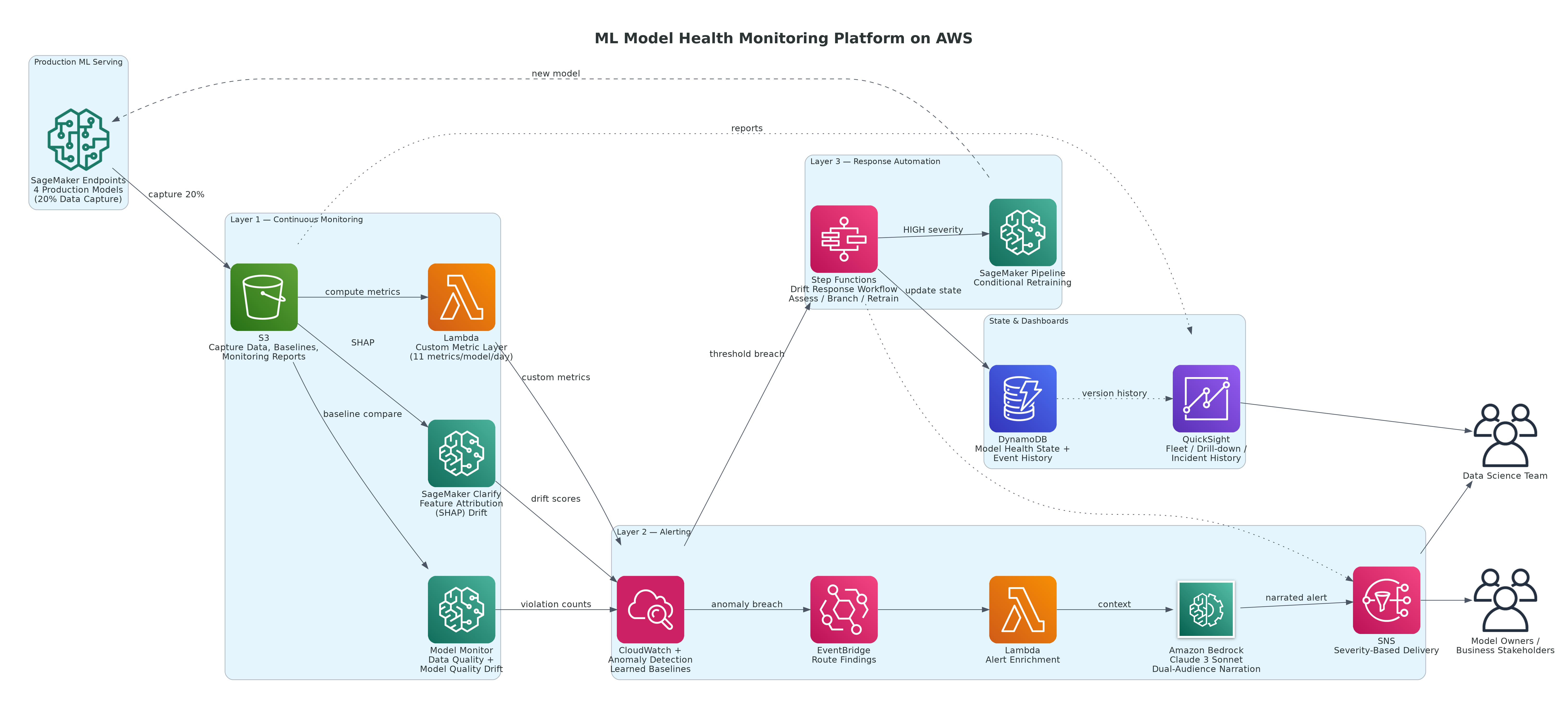
Figure 1: ML Model Health Monitoring Platform — Three-Layer Observability Architecture on AWS
AWS Services Used:
- Amazon SageMaker Model Monitor — automated data quality, model quality, feature attribution drift, and bias drift monitoring
- Amazon S3 — baseline statistics storage, monitoring reports, and model artifacts
- Amazon CloudWatch — custom metrics for prediction distribution, confidence score trends, and business-outcome correlation
- Amazon CloudWatch Anomaly Detection — ML-powered baseline for metric anomaly alerting
- Amazon EventBridge — routing Model Monitor findings to downstream alerting and response workflows
- AWS Lambda — custom metric computation, alert enrichment, and automated response triggers
- Amazon SNS — alert delivery to data science team, model owners, and business stakeholders
- Amazon QuickSight — model health dashboards with drill-down from fleet-level to individual feature level
- Amazon Bedrock (Claude 3 Sonnet) — natural language narration of drift findings for non-technical stakeholders
- Amazon DynamoDB — monitoring event history and model health state store
- AWS Step Functions — automated investigation and retraining trigger workflow
The architecture is organized into three layers: continuous monitoring that runs automatically against every production endpoint, alerting that routes findings to the right people at the right severity level, and response automation that initiates retraining when drift crosses defined thresholds.
Key Architectural Decisions
These are the decisions that shaped the monitoring platform — and the reasoning behind each one.
Decision 1: Why SageMaker Model Monitor Instead of Custom Monitoring Scripts?
When we began designing this platform, the data science team already had a collection of ad-hoc monitoring scripts — Python jobs that ran on a schedule, computed accuracy metrics against a sample of recent predictions, and emailed a CSV to a distribution list. The proposal to replace them with SageMaker Model Monitor initially met resistance: "We already have monitoring."
The gap was in what those scripts didn't catch. Custom accuracy scripts require ground truth labels — which for demand forecasting means waiting 30–90 days for actual sales data to come in before you can measure prediction accuracy. By the time the accuracy script fires an alert, the model has been making poor predictions for weeks.
SageMaker Model Monitor's data quality monitoring works on the input features themselves — no ground truth required. It detects when the distribution of inputs to the model has shifted away from the training baseline, which is an early warning signal for impending accuracy degradation, often days or weeks before accuracy metrics show it.
| Monitoring Type |
What It Catches |
Ground Truth Required |
Detection Lead Time |
| Custom accuracy scripts |
Accuracy drop after the fact |
Yes — often 30–90 day lag |
Days to weeks after degradation |
| SageMaker Data Quality Monitor |
Input feature distribution shift |
No |
Days before accuracy impact |
| SageMaker Model Quality Monitor |
Prediction accuracy vs. ground truth |
Yes |
When labels arrive |
| SageMaker Feature Attribution Drift |
SHAP value shifts across features |
No |
Days before accuracy impact |
| Custom CloudWatch metrics |
Business outcome correlation |
Partial |
Configurable |
The business decision: Data quality and feature attribution monitoring give you early warning before accuracy degrades. Accuracy monitoring tells you the model has already failed. For a business that makes decisions daily on model outputs, early warning is worth more than post-hoc confirmation.
Decision 2: Why Build a Custom Metric Layer on Top of Model Monitor?
SageMaker Model Monitor produces statistical monitoring reports — violations, constraint comparisons, distribution summaries. What it does not produce natively is business-aligned metrics: prediction confidence trend over the past 14 days, percentage of predictions in the high-confidence band vs. the uncertain band, correlation between model confidence and actual outcome accuracy, or the rolling 7-day prediction error by product category.
These are the metrics that business stakeholders can understand and act on. They are also the metrics that catch failure modes that statistical drift monitoring misses — specifically, cases where input distributions appear stable but the model's confidence is systematically shifting, which often precedes an accuracy drop on a specific segment of the data.
We built a Lambda-based custom metric layer that runs alongside Model Monitor, computing and publishing 11 custom CloudWatch metrics per model per day. CloudWatch Anomaly Detection then establishes a learned baseline for each metric and alerts when the metric deviates beyond the expected band.
The business decision: Statistical drift metrics are for data scientists. Business-outcome metrics are for the model owners who decide whether to retrain, adjust thresholds, or escalate. Both layers are necessary. Neither is sufficient alone.
Decision 3: Why Amazon Bedrock for Alert Narration?
A SageMaker Model Monitor violation report looks like this:
CODE
feature_name: units_sold_30d
constraint_check_type: distribution_statistics
description: Completeness check failed. Expected 0.98, Got 0.71
That output is actionable for a data scientist. It is not actionable for the demand planning manager who owns the model's business outcomes and needs to decide whether to hold a manual forecast review while the issue is investigated.
We added an Amazon Bedrock narration layer that converts Model Monitor violation reports and CloudWatch anomaly findings into plain-language summaries targeted at two audiences: a technical summary for the data science team and an executive summary for the model owner.
Example narration generated for a data quality violation on the demand forecasting model:
For the data science team: The units_sold_30d feature is showing 27% missing values in today's scoring batch, compared to a 2% baseline at training time. This is likely caused by a data pipeline upstream of the feature store — the feature relies on transaction data from the ERP integration, and the completeness drop coincides with the ERP maintenance window scheduled last night. Check the Glue ETL job for sales_transactions_daily before triggering retraining.
For the demand planning team: The demand forecasting model has detected an issue with one of its input data sources from last night. Today's predictions may be less reliable than usual for SKUs in the Electronics and Appliances categories. We recommend treating today's forecast output as indicative rather than definitive until the data science team confirms the issue is resolved — estimated by end of day.
That second paragraph is what prevents a business stakeholder from either ignoring a real issue or escalating a routine data pipeline hiccup into an emergency. It sets the right level of concern, in language that matches the audience, without requiring the data science team to write it manually for every alert.
The business decision: Monitoring without communication is incomplete. The alert needs to reach the right person with the right context and the right recommended action. Bedrock makes that possible at scale without manual effort.
Implementation Pattern
Setting Up SageMaker Model Monitor
Model Monitor requires three components per endpoint: a baseline computed from training data, a monitoring schedule that runs against live traffic, and a violation handler that routes findings downstream.
PYTHON
import boto3
import sagemaker
from sagemaker.model_monitor import (
    DefaultModelMonitor,
    DataCaptureConfig,
    CronExpressionGenerator
)
from sagemaker.model_monitor.dataset_format import DatasetFormat

sagemaker_session = sagemaker.Session()
role = sagemaker.get_execution_role()
bucket = "ml-monitoring-bucket"
endpoint_name = "demand-forecast-endpoint-prod"

# Step 1: Enable data capture on the endpoint
# This captures a sample of inference requests and responses to S3
data_capture_config = DataCaptureConfig(
    enable_capture=True,
    sampling_percentage=20,          # Capture 20% of traffic — sufficient for drift detection
    destination_s3_uri=f"s3://{bucket}/data-capture/{endpoint_name}",
    capture_options=["Input", "Output"],
    csv_content_types=["text/csv"],
    json_content_types=["application/json"]
)

# Apply to endpoint — update in place, no redeployment required
predictor = sagemaker.predictor.Predictor(
    endpoint_name=endpoint_name,
    sagemaker_session=sagemaker_session
)
predictor.update_data_capture_config(data_capture_config=data_capture_config)

# Step 2: Compute baseline statistics from training data
monitor = DefaultModelMonitor(
    role=role,
    instance_count=1,
    instance_type="ml.m5.xlarge",
    volume_size_in_gb=20,
    max_runtime_in_seconds=3600,
    sagemaker_session=sagemaker_session
)

monitor.suggest_baseline(
    baseline_dataset=f"s3://{bucket}/training-data/baseline.csv",
    dataset_format=DatasetFormat.csv(header=True),
    output_s3_uri=f"s3://{bucket}/baseline-results/{endpoint_name}",
    wait=True
)

# Step 3: Create daily monitoring schedule
monitor.create_monitoring_schedule(
    monitor_schedule_name=f"{endpoint_name}-data-quality-monitor",
    endpoint_input=endpoint_name,
    output_s3_uri=f"s3://{bucket}/monitoring-reports/{endpoint_name}",
    statistics=monitor.baseline_statistics(),
    constraints=monitor.suggested_constraints(),
    schedule_cron_expression=CronExpressionGenerator.daily(),
    enable_cloudwatch_metrics=True      # Publish violation counts to CloudWatch
)
Feature attribution drift monitoring runs in parallel using SageMaker Clarify, tracking SHAP value distributions across features to detect when the model's reliance on specific features has shifted — a subtler but often more informative signal than raw data distribution drift.
PYTHON
from sagemaker.clarify import (
    SageMakerClarifyProcessor,
    ModelConfig,
    ModelPredictedLabelConfig,
    SHAPConfig,
    DataConfig
)

clarify_processor = SageMakerClarifyProcessor(
    role=role,
    instance_count=1,
    instance_type="ml.m5.xlarge",
    sagemaker_session=sagemaker_session
)

shap_config = SHAPConfig(
    baseline=[
        # Baseline values for each feature — use training set means
        [2847, 0.73, 14.2, 3, 1, 0.91, 28, 0, 1, 0.84]
    ],
    num_samples=500,
    agg_method="mean_abs",
    save_local_shap_values=False
)

clarify_processor.run_explainability(
    data_config=DataConfig(
        s3_data_input_path=f"s3://{bucket}/data-capture/{endpoint_name}/recent/",
        s3_output_path=f"s3://{bucket}/explainability/{endpoint_name}",
        label="prediction",
        dataset_type="text/csv"
    ),
    model_config=ModelConfig(
        model_name="demand-forecast-model-v4",
        instance_type="ml.m5.xlarge",
        instance_count=1
    ),
    explainability_config=shap_config
)
Custom CloudWatch Metric Layer
The Lambda function runs daily after Model Monitor completes, pulling the captured inference data from S3, computing business-aligned metrics, and publishing them to CloudWatch under a custom namespace.
PYTHON
import boto3
import json
import numpy as np
from datetime import datetime, timedelta

s3 = boto3.client("s3")
cloudwatch = boto3.client("cloudwatch", region_name="ap-south-1")

def compute_and_publish_model_metrics(endpoint_name: str, bucket: str):
    """
    Compute business-aligned health metrics from captured inference data
    and publish to CloudWatch for anomaly detection and dashboarding.
    """
    # Load last 24 hours of captured inference data from S3
    prefix = f"data-capture/{endpoint_name}/{datetime.utcnow().strftime('%Y/%m/%d')}/"
    response = s3.list_objects_v2(Bucket=bucket, Prefix=prefix)

    predictions = []
    confidence_scores = []

    for obj in response.get("Contents", []):
        data = json.loads(
            s3.get_object(Bucket=bucket, Key=obj["Key"])["Body"].read()
        )
        for record in data.get("captureData", {}).get("endpointOutput", {}).get("data", []):
            pred = float(record.get("prediction", 0))
            conf = float(record.get("confidence", 0))
            predictions.append(pred)
            confidence_scores.append(conf)

    if not predictions:
        return

    metrics = [
        # % of predictions in high-confidence band (>0.80)
        {
            "MetricName": "HighConfidencePredictionRate",
            "Value": sum(1 for c in confidence_scores if c > 0.80) / len(confidence_scores),
            "Unit": "None"
        },
        # Mean confidence score — a downward trend precedes accuracy drops
        {
            "MetricName": "MeanPredictionConfidence",
            "Value": float(np.mean(confidence_scores)),
            "Unit": "None"
        },
        # Coefficient of variation — unusually high variance signals instability
        {
            "MetricName": "PredictionCoefficientOfVariation",
            "Value": float(np.std(predictions) / np.mean(predictions))
                     if np.mean(predictions) != 0 else 0,
            "Unit": "None"
        },
        # Predictions outside historical interquartile range — outlier rate
        {
            "MetricName": "OutOfRangePredictionRate",
            "Value": sum(
                1 for p in predictions
                if p < np.percentile(predictions, 5) or p > np.percentile(predictions, 95)
            ) / len(predictions),
            "Unit": "None"
        }
    ]

    cloudwatch.put_metric_data(
        Namespace=f"MLModelHealth/{endpoint_name}",
        MetricData=[
            {**m, "Timestamp": datetime.utcnow(), "Dimensions": [
                {"Name": "EndpointName", "Value": endpoint_name},
                {"Name": "Environment", "Value": "production"}
            ]}
            for m in metrics
        ]
    )
CloudWatch Anomaly Detection is then configured on each custom metric to establish a learned band based on 14 days of history. When a metric breaches the anomaly band, EventBridge routes the finding to the alert enrichment Lambda, which queries the monitoring history, assembles context, and calls Bedrock for narration before dispatching to SNS.
Bedrock Alert Narration
PYTHON
import boto3
import json

bedrock = boto3.client("bedrock-runtime", region_name="ap-south-1")

def narrate_drift_alert(alert_context: dict) -> dict:
    """
    Convert raw monitoring findings into plain-language summaries
    for two audiences: data science team and business model owner.
    """
    prompt = f"""You are an ML observability analyst. A production model health alert has been triggered.

Alert Details:
- Model: {alert_context['model_name']}
- Endpoint: {alert_context['endpoint_name']}
- Alert type: {alert_context['alert_type']}
- Triggered metric: {alert_context['metric_name']}
- Current value: {alert_context['current_value']}
- Expected range: {alert_context['expected_range']}
- Violation summary from SageMaker Model Monitor: {alert_context['violations']}
- Recent business context: {alert_context['business_context']}
- Model purpose: {alert_context['model_purpose']}

Write two summaries:

1. TECHNICAL SUMMARY (for the data science team): Explain what metric triggered, what it likely means technically, what to investigate first, and whether retraining is likely needed. Be specific.

2. BUSINESS SUMMARY (for the model owner): Explain in plain language what is happening, how it might affect decisions made using this model today, and what action they should take (if any) while the team investigates. Avoid technical jargon. Maximum 3 sentences.

Respond as a JSON object with keys: technical_summary (string), business_summary (string), recommended_action (string: one of INVESTIGATE, RETRAIN, ESCALATE, MONITOR)."""

    response = bedrock.invoke_model(
        modelId="anthropic.claude-3-sonnet-20240229-v1:0",
        contentType="application/json",
        accept="application/json",
        body=json.dumps({
            "anthropic_version": "bedrock-2023-05-31",
            "max_tokens": 600,
            "temperature": 0.1,     # Very low temperature — consistent, factual narration
            "messages": [{"role": "user", "content": prompt}]
        })
    )

    result = json.loads(response["body"].read())
    return json.loads(result["content"][0]["text"])
Automated Response: Step Functions Retraining Workflow
When drift severity crosses a defined threshold — specifically, when data quality violations exceed 15% of monitored features or feature attribution drift exceeds 0.25 on any top-5 SHAP feature — Step Functions triggers an automated investigation and conditional retraining workflow.
CODE
CloudWatch Alarm (drift threshold breached)
    → EventBridge rule
    → Step Functions: ModelDriftResponseWorkflow
        → State 1: AssessViolationSeverity
              Query Model Monitor reports from last 3 days
              Compute trend: is drift accelerating or stable?
        → State 2 (branch on severity):
              LOW: Publish enhanced monitoring alert, increase
                   capture sampling to 50%, notify data science team
              MEDIUM: Trigger data validation job on feature store,
                      notify model owner + data science team,
                      schedule retraining review in 48 hours
              HIGH: Trigger SageMaker Pipeline retraining immediately,
                    notify all stakeholders, flag predictions
                    as "under review" in the serving layer
        → State 3: UpdateModelHealthState (DynamoDB)
        → State 4: NotifyStakeholders (SNS → Bedrock narration)
This workflow means that a high-severity drift event triggers an automatic retraining run without requiring a data scientist to manually initiate it at 2am — while still routing appropriate notifications so the team can validate the retrained model before it goes live.
QuickSight Model Health Dashboard
The QuickSight dashboard consumes data from three sources: Model Monitor reports stored in S3, custom CloudWatch metrics exported via a Lambda-based ETL to S3, and model version history stored in DynamoDB. It is organized in three views:
- Fleet view: All four production models at a glance, with a RAG (Red/Amber/Green) health status for each based on composite drift score. The first screen any data science team member sees in the morning.
- Model drill-down: Per-model view showing data quality violation trend (30 days), feature attribution drift per feature (heatmap), confidence score trend, and prediction distribution vs. training baseline.
- Incident history: Timeline of all drift alerts, the Bedrock-generated narratives, actions taken, and time-to-resolution — building the audit trail that compliance and leadership need.
Cost Architecture and AWS Service Spend
At steady-state monitoring four production SageMaker endpoints with daily monitoring schedules:
| Service |
Usage |
Estimated Monthly Cost |
| SageMaker Model Monitor |
4 endpoints × daily schedule, ml.m5.xlarge processing |
~$96 |
| SageMaker Clarify (SHAP drift) |
4 runs/week × ml.m5.xlarge |
~$58 |
| Amazon S3 |
~180 GB (capture data, reports, baselines) |
~$4 |
| Amazon CloudWatch |
44 custom metrics, anomaly detection on 16 metrics, 120 alarms |
~$38 |
| AWS Lambda |
~180K invocations/month (metric computation + alert enrichment) |
~$2 |
| Amazon Bedrock (Claude 3 Sonnet) |
~60 narration calls/month (alert events only) |
~$1 |
| AWS Step Functions |
~12 workflow executions/month |
~$1 |
| Amazon SNS |
~200 alert notifications/month |
~$1 |
| Amazon QuickSight |
3 authors, 8 readers |
~$54 |
| Amazon DynamoDB |
Monitoring state store, low volume |
~$3 |
| Total |
|
~$258/month |
The cost profile is dominated by SageMaker processing instances running the monitoring jobs. The Bedrock narration cost is negligible — approximately $1/month for the volume of alerts a healthy production ML platform generates — because Bedrock is only invoked when a real alert fires, not on every monitoring run.
Against the cost of one silent drift incident — the retail client's demand forecasting drift resulted in an estimated ₹28–34 lakh in suboptimal inventory positioning over the 11 weeks it went undetected — the monitoring platform's infrastructure cost is recovered in the first incident it prevents.
Common Pitfalls (Real Lessons)
| Pitfall |
What Happened |
How We Fixed It |
| Baseline computed on a small training sample |
Model Monitor flagged 60% of features as drifted on day one — all false positives |
Recomputed baseline on full training dataset; minimum 10,000 records required |
| Alert thresholds set too tight on high-variance features |
PagerDuty fatigue — team started ignoring alerts within two weeks |
Analyzed 30-day metric history before setting thresholds; applied percentile-based bands not fixed values |
| Data capture at 100% sampling |
S3 storage costs ballooned to $340/month in week one |
Set sampling to 20% — statistically sufficient for drift detection at our volumes |
| Step Functions retraining triggered on a data pipeline outage |
Model retrained on 3 days of incomplete data, performance regressed |
Added data completeness gate before retraining trigger: >95% feature completeness required |
| QuickSight dashboard showed raw violation counts |
Business stakeholders interpreted every violation as a crisis |
Changed primary metric to composite health score (0–100) with clear RAG thresholds and plain-language status descriptions |
Each of these mistakes was instructive. The hardest lesson was the alert threshold problem — a monitoring system that people stop reading is worse than no monitoring at all, because it creates a false sense of coverage while providing none.
Business Outcomes
| Metric |
Before |
After |
Business Impact |
| Mean time to detect model degradation |
~47 days |
< 72 hours |
Drift caught before business decisions are affected |
| Monitoring coverage |
1 of 4 models (ad hoc) |
4 of 4 models (automated, continuous) |
Full production fleet visibility |
| Data science time on reactive investigation |
~35% of sprint capacity |
~8% of sprint capacity |
Freed for model improvement work |
| Silent drift incidents (annualised) |
3 known, unknown unknowns |
0 since platform launch |
Planning team trust in model outputs restored |
| Stakeholder alert actionability |
Raw violation reports — ignored |
Bedrock-narrated, audience-targeted alerts |
Right action taken within 4 hours of alert |
| Compliance audit readiness |
No documentation trail |
Full incident history with actions and resolutions |
Audit-ready model governance record |
The most significant shift was not technical — it was cultural. Before the monitoring platform, the data science team was in a reactive posture: something would break, someone would complain, the team would investigate. After the platform, the team is in a proactive posture: the system alerts them to an emerging issue, they investigate and resolve it before it surfaces as a business complaint. That shift from reactive to proactive is the organizational value of model observability, and it doesn't appear on an AWS cost report.
Lessons for Technology Leaders
- A model that produces predictions without health visibility is a liability, not an asset — Every ML model in production is making a claim about the world. As the world changes, that claim becomes less reliable. Without continuous monitoring, you have no way to know when to stop trusting it — and neither does the business.
- Data quality monitoring is more valuable than accuracy monitoring for models with delayed ground truth — If your model's outcomes take weeks or months to observe, waiting for accuracy metrics means waiting for the damage to be done. Monitor the inputs. Input distribution shift is an early warning signal for accuracy degradation — often days or weeks ahead of the accuracy drop itself.
- Monitoring thresholds must be calibrated on real traffic, not set by intuition — Thresholds set too tight create alert fatigue and teams that ignore monitoring. Thresholds set too loose miss real issues. Spend the time analyzing 30 days of metric history before setting any threshold. The time investment pays back in monitoring that people actually trust and act on.
- Alert communication is a product, not a side effect — An alert that a data scientist understands but a business stakeholder ignores is a monitoring failure. Invest in audience-targeted communication. The Bedrock narration layer added minimal cost and dramatically changed how quickly appropriate actions were taken on drift events.
- Automated response is the destination, not the starting point — Start with alerting. Add dashboards. Build stakeholder trust in the monitoring data. Only then introduce automated retraining triggers — once the team has validated that the monitoring signals are reliable enough to act on autonomously. Automation built on unvalidated signals creates more problems than it solves.
About the Author
Chandni Gadhvi is Program Manager – Data and AI at AeonX Digital Technology Limited, where she leads the architecture and delivery of cloud-native AI and MLOps solutions for enterprise customers. She specializes in building production-grade ML systems on AWS that are observable, governable, and continuously improving. She is an advocate for operationally mature AI — the kind that earns and keeps business trust over time — and shares technical thought leadership to help engineering teams close the gap between ML in development and ML in production.
by Chandni Gadhvi | Apr 15, 2026 | AWS
The Quality Intelligence Imperative: Why Manual Inspection Is a Manufacturing Risk
In high-volume manufacturing, quality inspection is one of the last processes to be digitally transformed — and often one of the most expensive when it isn't.
The reason manual inspection persists is understandable: it feels controllable. You can see the inspectors working, count the headcount, measure attendance. What you cannot easily measure is the inspection you missed on the 200th unit at the end of a shift, the subtle assembly defect that gets through because two inspectors interpreted the standard differently, or the batch-level failure that could have been caught at the individual unit level if your data had been structured enough to see the pattern forming.
When we engaged with an automotive component manufacturer facing these challenges, the gap between their inspection model and their quality outcomes was measurable and expensive: 82% inspection accuracy with 100% manual coverage, a defect escape rate that was generating warranty claims and OEM escalations, and no digital record of what had been inspected, when, or by whom.
The problem wasn't effort — the inspection team was working. The problem was that manual inspection at production speed is physiologically limited. Human attention degrades with volume, lighting variation, shift fatigue, and cognitive load. AI does not have those constraints.
This post documents how we designed and deployed a real-time AI-powered visual inspection platform for that manufacturer — combining YOLOv11 edge inference with Amazon Bedrock's generative intelligence and AWS IoT-based cloud ingestion to deliver what manual inspection could not: consistent, traceable, continuously improving quality coverage at full production speed.
As Technical Architect for this initiative at AeonX Digital, I led the architecture design, model strategy, and AWS service selection across the edge and cloud layers. What follows covers the implementation in enough detail to be useful to practitioners, along with the architectural decisions and trade-offs that shaped each choice.
The outcome: inspection accuracy increased from 82% to 97%, quality-related costs reduced by approximately 35% annually, and the manufacturer moved from sample-based inspection to full AI-driven coverage on every unit produced.
Why This Matters Now: The Edge AI Inflection Point in Manufacturing
Three forces are converging to make AI-powered inspection a mainstream manufacturing capability rather than a pilot project:
- Edge compute has reached production-grade reliability — NVIDIA Jetson AGX Orin and similar edge AI platforms now deliver inference speeds that match assembly line cycle times. The latency barrier that made cloud-only AI inspection impractical is gone. Inference happens at the device, in single-digit milliseconds, with no dependency on network connectivity for the primary quality decision.
- Computer vision models have matured for industrial use — Transfer learning from large pretrained models like YOLO architectures means that a manufacturer no longer needs tens of thousands of defect images to build a high-accuracy detector. Fine-tuning on a few thousand labeled images now produces production-grade accuracy in days, not months.
- Generative AI closes the gap between detection and action — Traditional computer vision tells you what it found. It doesn't tell you what to do about it. Amazon Bedrock converts detection outputs into plain-language summaries, corrective action recommendations, and trend narratives that a plant supervisor can act on without interpreting bounding boxes and confidence scores.
The decision to build this system was driven by a quality leadership team that recognized manual inspection was no longer scaling with production volume — and that the cost of escaped defects had begun to exceed the cost of building a better system.
The Business Problem
The manufacturer's existing inspection workflow had:
- 100% manual inspection with no structured defect criteria — consistent judgment depended entirely on individual inspector experience
- No real-time alerting — defect patterns were visible only in end-of-shift reports, after hundreds of units had already been produced
- No digital audit trail per unit — traceability for OEM compliance was manual and incomplete
- No predictive capability — root cause analysis happened after warranty claims, not before
- Sample-based documentation — only a fraction of inspected units had any recorded evidence
Business impact of the status quo:
- Rising rework costs from defects caught late in the production process
- OEM escalations and warranty claims from defects caught by customers
- Inability to scale inspection headcount proportionally with production volume increases
- Compliance exposure from incomplete traceability records
The goal was not to assist manual inspection — it was to replace it with a system that was faster, more consistent, and fully traceable, while keeping quality engineers in the loop as analysts rather than inspectors.
Technical Architecture: Edge + Cloud + GenAI
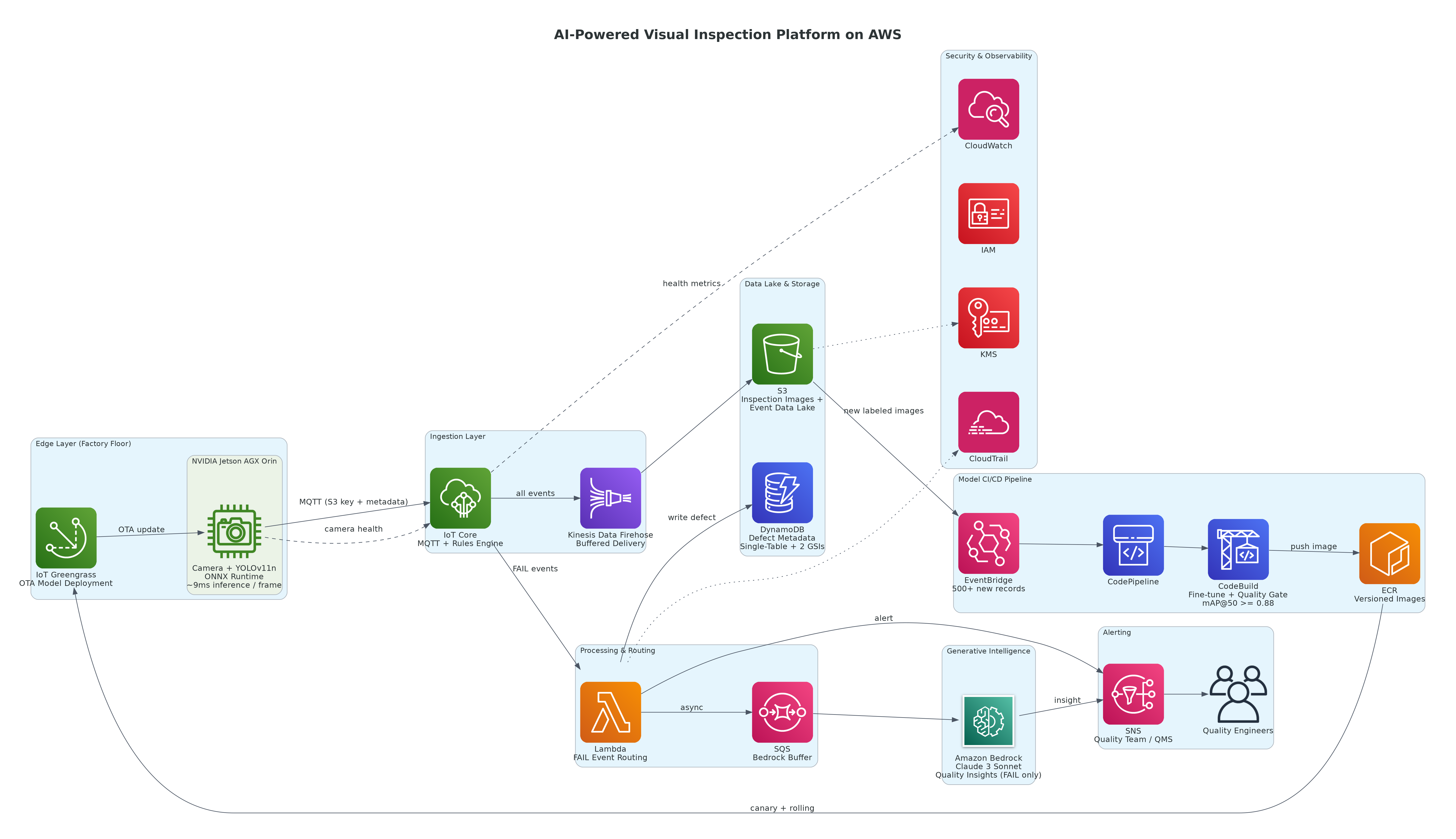
Figure 1: AI-Powered Visual Inspection Platform — Edge + Cloud + GenAI Reference Architecture
AWS and Technology Stack:
- YOLOv11n (Ultralytics) — custom-trained object detection models on NVIDIA Jetson AGX Orin edge devices
- ONNX Runtime — edge inference engine for runtime-agnostic deployment
- AWS IoT Core — secure MQTT ingestion from edge to cloud
- Amazon Kinesis Data Firehose — buffered delivery to S3 data lake
- Amazon S3 — inspection image and event data lake
- Amazon DynamoDB — structured defect metadata with single-table design
- Amazon Bedrock (Claude 3 Sonnet) — generative quality insights for FAIL events
- Amazon SNS — real-time alerting to quality teams and QMS
- AWS IoT Greengrass — OTA model deployment to edge devices
- AWS CodePipeline + Amazon ECR — automated model retraining and deployment pipeline
- Amazon CloudWatch and CloudTrail — observability and compliance audit
- AWS KMS and IAM — encryption and access control
The architecture combines three layers: edge inference for latency-critical pass/fail decisions, cloud data lake for analytics and model retraining, and generative AI for converting detections into actionable insights. Each layer was designed to be independently scalable and replaceable.
Key Architectural Decisions
Decision 1: Why Edge Inference Instead of Cloud Inference?
The first architectural question for any computer vision deployment in manufacturing is where inference runs. Cloud inference is simpler to operate — you push images to an API and get results back. The problem is latency.
At five units per minute on an assembly line, the maximum acceptable inspection-to-decision time is 180ms. A round-trip cloud API call — accounting for image upload, inference, and response — consistently exceeds 300–400ms under normal network conditions, and is completely unavailable during network interruptions.
Edge inference on NVIDIA Jetson AGX Orin with ONNX Runtime delivers 9ms per frame. That is not incremental improvement over cloud inference — it is a fundamentally different latency class that makes real-time line-speed inspection possible.
| Approach |
Inference Latency |
Network Dependency |
Cost at Scale |
| Cloud inference (API) |
300–400ms |
Hard dependency |
High — every frame billed |
| Edge inference (ONNX) |
~9ms |
None for primary decision |
Low — compute is local |
| Edge inference (TensorRT FP16) |
~4.5ms |
None |
Low — optimized for device |
The business decision: Production lines do not pause for network issues. Edge inference removes the network from the critical path for the primary quality decision. Cloud connectivity is required for analytics, alerting, and model updates — but not for the inspection itself.
Decision 2: Why YOLOv11n Over Larger Model Variants?
We benchmarked three YOLOv11 variants during model selection:
- YOLOv11n (nano): mAP@50 of 0.91 after fine-tuning, 9ms inference latency on Jetson AGX Orin
- YOLOv11s (small): mAP@50 of 0.94, 21ms inference latency
- YOLOv11m (medium): mAP@50 of 0.96, 38ms inference latency
The 3–5 percentage point accuracy improvement from larger models was real but insufficient to justify the latency trade-off. At 5 units per minute, 21ms is already marginal headroom. At 38ms, the model cannot keep pace with line speed at all production rates. YOLOv11n at 9ms gives 20× headroom over cycle time — sufficient buffer for device temperature variation, I/O overhead, and future production rate increases.
The business decision: Accuracy matters, but availability matters more. A model with 91% mAP that runs reliably at every production rate is more valuable than a 96% mAP model that creates line stoppages during rate increases.
The defect metadata workload is write-intensive: at 72,000 inspections per day across three production lines, the system generates sustained write throughput with short burst peaks during production starts and end-of-line inspections.
We evaluated Aurora PostgreSQL first, given the team's familiarity with SQL. The decision shifted to DynamoDB for three specific reasons:
- Burst write handling without connection pooling — RDS connection pools become a bottleneck under burst write conditions. DynamoDB on-demand capacity handles burst transparently without connection management overhead.
- Access patterns were well-defined — The three primary query patterns (by product unit, by station + time range, by shift + defect class) mapped cleanly to a single-table design with two GSIs. No ad-hoc joins were required.
- TTL-based retention — Compliance required one-year defect record retention followed by automatic deletion. DynamoDB's native TTL feature handles this without a separate archival job.
The business decision: DynamoDB's operational simplicity at the write volumes this workload generates outweighed Aurora's query flexibility for access patterns that are well-understood in advance.
Implementation Pattern
YOLOv11 Model Training: Dataset and Configuration
Model training was the most labor-intensive phase of the project. The dataset comprised 11,400 labeled images across six defect classes: missing fastener, misaligned bracket, incorrect cable routing, surface scratch, incomplete weld, and foreign object presence. Annotation was performed in CVAT with double-blind review by quality engineers to ensure label consistency across inspectors.
PYTHON
from ultralytics import YOLO

# Fine-tune YOLOv11n on defect dataset
model = YOLO("yolo11n.pt")  # COCO-pretrained base weights

results = model.train(
    data="defect_dataset.yaml",    # Class names, train/val/test paths
    epochs=100,
    imgsz=640,
    batch=16,
    device="cuda:0",               # NVIDIA Jetson AGX Orin (2048 CUDA cores)
    optimizer="AdamW",
    lr0=0.001,
    lrf=0.01,
    momentum=0.937,
    weight_decay=0.0005,
    augment=True,
    patience=15,                   # Early stopping — critical for small defect classes
    cos_lr=True,                   # Cosine LR decay — more stable fine-tuning
    project="quality_inspection",
    name="yolov11_defect_v3",
    save=True,
    val=True
)

# Export to ONNX for runtime-agnostic edge deployment
model.export(format="onnx", dynamic=True, simplify=True)
Model performance after fine-tuning:
| Metric |
COCO Pretrained Only |
Fine-tuned v3 |
| mAP@50 |
0.58 |
0.91 |
| mAP@50-95 |
0.39 |
0.77 |
| Precision |
0.71 |
0.93 |
| Recall |
0.65 |
0.90 |
| Inference latency (Jetson AGX Orin, ONNX) |
~6ms |
~9ms |
Data augmentation — horizontal flip, brightness jitter (±20%), random rotation (±5°), and mosaic augmentation — was essential for handling ambient lighting variation across three production shifts. Without augmentation, the model performed well under optimal lighting and poorly in early morning conditions when production lighting takes time to stabilize.
Secure IoT Ingestion: MQTT Topic Design
CODE
manufacturing/{plant_id}/line/{line_id}/station/{station_id}/inspection
manufacturing/{plant_id}/line/{line_id}/station/{station_id}/camera/health
manufacturing/{plant_id}/alerts/defects
Each inspection event published to IoT Core:
JSON
{
  "event_id": "insp-20241118-STN12-04231",
  "timestamp": "2024-11-18T08:43:17.823Z",
  "plant_id": "PLANT-MH-01",
  "line_id": "LINE-03",
  "station_id": "STN-12",
  "product_id": "PROD-VAR-B-00892",
  "inspection_result": "FAIL",
  "defects": [
    {
      "class": "missing_fastener",
      "confidence": 0.91,
      "bounding_box": [412, 318, 56, 48]
    }
  ],
  "model_version": "yolov11_defect_v3",
  "inference_latency_ms": 9,
  "image_s3_key": "inspections/2024/11/18/LINE-03/STN-12/insp-04231.jpg"
}
IoT device policies enforced least-privilege — each edge device could publish only to its own station topic hierarchy, preventing cross-station data injection. IoT Core rules engine routed all events to Kinesis Data Firehose for S3 delivery, FAIL events additionally to Lambda for DynamoDB write and SNS alert, and camera health events to CloudWatch metrics.
DynamoDB Single-Table Design
PYTHON
import boto3
from datetime import datetime

dynamodb = boto3.resource("dynamodb", region_name="ap-south-1")
table = dynamodb.Table("QualityInspectionEvents")

def record_defect(event: dict):
    table.put_item(
        Item={
            # PK/SK: lookup by product unit for traceability report
            "PK": f"PRODUCT#{event['product_id']}",
            "SK": f"INSPECTION#{event['timestamp']}",

            # GSI-1: station + time range for root cause analysis
            "GSI1PK": f"STATION#{event['station_id']}",
            "GSI1SK": event["timestamp"],

            # GSI-2: shift + defect class for quality dashboard aggregation
            "GSI2PK": f"SHIFT#{event['shift_id']}",
            "GSI2SK": f"CLASS#{event['defects'][0]['class']}",

            "inspection_result": event["inspection_result"],
            "defects": event["defects"],
            "model_version": event["model_version"],
            "image_s3_key": event["image_s3_key"],
            "plant_id": event["plant_id"],
            "line_id": event["line_id"],
            "ttl": int(datetime.now().timestamp()) + (365 * 24 * 3600)
        }
    )
Generative AI Interpretation: Bedrock on FAIL Events Only
Traditional computer vision tells plant supervisors what was detected. Amazon Bedrock tells them what to do about it.
We integrated Bedrock only for FAIL inspection events — approximately 14% of total volume. This keeps Bedrock spend proportional to business value: a PASS result requires no natural language explanation.
Example: a missing fastener detection at Station 12 produces the following Bedrock output:
"Fastener A missing at Station 12 (confidence 91%). Pattern matches three prior events on LINE-03 this shift — likely feeder misalignment rather than isolated miss. Recommend pausing LINE-03 for feeder inspection before producing additional units on Variant B."
That recommendation was not possible from computer vision output alone. It requires correlating the current detection against the session history — which is passed as context in the Bedrock prompt — to surface the pattern rather than the isolated event.
CI/CD Pipeline: OTA Model Deployment to Edge
CODE
S3 (new labeled defect images, threshold: 500+ new records)
    → EventBridge rule
    → CodePipeline triggered
        → CodeBuild: validate labels, merge with training set
        → CodeBuild: fine-tune YOLOv11n (100 epochs, ~45 min on ml.g4dn.xlarge spot)
        → Quality gate: mAP@50 ≥ 0.88
            → FAIL: SNS alert to ML team, pipeline stops
            → PASS: export ONNX, build Docker image
        → ECR: push versioned image (e.g., yolov11-defect:v4.1)
        → IoT Greengrass: create new component version
        → Canary: deploy to 2 of 12 edge devices, monitor 30 minutes
            → Drift detected: auto-rollback to previous ECR tag
            → Healthy: rolling update to remaining 10 devices
End-to-end from data trigger to full fleet update: approximately 3.5 hours. This replaced a manual process where model updates required SSH access to edge devices and happened quarterly at best — meaning newly introduced product variants ran uninspected on existing models for weeks before anyone noticed the accuracy degradation.
Cost Architecture and AWS Infrastructure Spend
At steady-state processing approximately 72,000 inspections per day (three production lines, single-shift, 20 working days per month):
| Service |
Usage |
Estimated Monthly Cost |
| AWS IoT Core |
~1.44M messages/month at $1.00/M |
~$1.44 |
| Kinesis Data Firehose |
~14 GB/month ingested |
~$4 |
| Amazon S3 |
~2.2 TB stored (inspection images + data lake) |
~$51 |
| Amazon DynamoDB |
~1.44M writes/day on-demand at $0.625/M WRU |
~$27 |
| Amazon Bedrock (Claude 3 Sonnet) |
~10,000 FAIL events/month, avg 600 input + 300 output tokens |
~$63 |
| Amazon SNS |
~12K alerts/month |
~$1 |
| AWS Lambda |
~2.4M invocations/month, 256MB memory |
~$9 |
| CodePipeline + ECR |
2 pipelines, ~20 GB image storage |
~$18 |
| IoT Greengrass |
12 core devices |
~$18 |
| CloudWatch + CloudTrail |
Custom metrics, log ingestion, audit |
~$34 |
| Total |
|
~$226/month |
If Bedrock had been invoked on every inspection event rather than FAIL events only, monthly Bedrock spend would increase to approximately $450/month with no incremental business value. Filtering at the Lambda routing layer keeps GenAI spend proportional to actual need.
Against the approximately 35% reduction in quality-related costs — warranty claims, rework labour, and OEM penalty charges — the AWS infrastructure at approximately ₹19,000 per month is a rounding error on the ROI calculation.
Common Pitfalls (Real Lessons)
| Pitfall |
What Happened |
How We Fixed It |
| Model trained on controlled lighting images only |
Accuracy dropped to 74% on night shift |
Added brightness jitter and shift-stratified dataset sampling |
| IoT Core message size exceeded 128KB limit |
Large image metadata payloads failed silently |
Moved image to S3 first, sent only S3 key in MQTT payload |
| Greengrass deployment without canary stage |
A broken model update halted inspection on all 12 devices simultaneously |
Added 2-device canary with 30-minute observation window before fleet rollout |
| Bedrock called synchronously in Lambda |
FAIL events during production bursts created queue backlog |
Moved to async Lambda invocation with SQS buffer for Bedrock calls |
These emerged in production, not in testing. Documenting them in your runbook before they repeat is the operational habit that separates mature ML systems from perpetual firefighting.
Business Outcomes
| Metric |
Before |
After |
Business Impact |
| Inspection accuracy |
82% |
97% |
Defect escape rate reduced significantly |
| Inspection coverage |
Sample-based |
100% of units |
Full traceability per unit |
| Quality-related costs |
Baseline |
~35% reduction |
Warranty and rework savings |
| Defect detection speed |
End-of-shift report |
Real-time (<180ms per unit) |
Prevents batch-level failures |
| Audit traceability |
Manual, incomplete |
Full digital record per unit |
OEM compliance confidence |
| Inspector redeployment |
100% on line inspection |
Shifted to quality analysis |
Higher-value work per head |
The most significant shift was not the accuracy improvement — it was the move from reactive to preventive quality management. Under the manual system, defect patterns were visible only after they had produced a batch of defective units. Under the AI system, a pattern forming at Station 12 across 8 units in a 30-minute window triggers an alert before it becomes a batch failure. That early warning capability is the real value of real-time inspection — and it was not possible without structured, timestamped, per-unit data at production speed.
Lessons for Technology Leaders
- Edge inference is not optional for production-speed applications — Cloud inference introduces latency and network dependency that manufacturing environments cannot accept. The decision between edge and cloud is not a preference — it is a function of cycle time requirements. Measure your cycle time before you choose your inference architecture.
- Model selection is a latency decision, not an accuracy decision — The difference between YOLOv11n and YOLOv11s in accuracy is 3 percentage points. The difference in latency is 12ms. At production scale, the latency gap closes the conversation. Start with the latency constraint and work backwards to the model.
- GenAI enhances CV outputs — it doesn't replace structured data — The Bedrock recommendations that resonated most with the quality team were the ones that correlated current detections against session history. That correlation requires structured, queryable defect data in DynamoDB. GenAI without a data layer is a demo. GenAI with a data layer is a tool.
- OTA deployment is an operational requirement, not a feature — A model that cannot be updated remotely will degrade silently as product variants change and lighting conditions shift. Build the OTA pipeline before the first production model deployment, not after you've experienced the first degradation incident.
- Model governance is a compliance requirement in regulated manufacturing — Per-unit model version logging, automated rollback, and quarterly review processes are not engineering overhead — they are the audit evidence that quality leadership and OEM customers need to trust AI-driven pass/fail decisions.
About the Author
Chandni Gadhvi is Program Manager – Data and AI at AeonX Digital Technology Limited, where she leads the architecture and delivery of cloud-native AI and computer vision solutions for industrial enterprises. She specializes in edge-to-cloud AI systems on AWS that convert real-time operational data into quality intelligence. She is an advocate for practical AI deployment in manufacturing and shares technical thought leadership to help engineering teams move from proof-of-concept to production-grade systems on AWS.
by Chandni Gadhvi | Apr 1, 2026 | AWS
The Freight Intelligence Imperative: Why Manual Logistics Is a Business Risk
In large industrial enterprises, freight management is rarely treated as a strategic problem. It gets managed as an operational one — spreadsheets, phone calls, and planners who negotiate rates based on intuition built over years of experience.
That model worked when freight spend was stable and predictable. It breaks when you're processing hundreds of bookings a month across dozens of routes, managing fifteen-plus vendors with variable SLA histories, and operating in a market where fuel prices, seasonal demand, and carrier capacity shift faster than any spreadsheet can track.
When we engaged with an enterprise manufacturing organization facing these challenges, the symptoms were familiar: freight costs running 20–25% above industry benchmarks, booking cycles averaging four days, and no structured way to know which vendor to trust for a given route until after the delivery had either arrived on time or not. The organization had no centralized freight data, no predictive capability, and no way to learn from historical performance at scale.
The real problem wasn't that they lacked technology — they had an ERP. The problem was that their logistics decisions were disconnected from their data. Every booking was effectively made from scratch.
This post documents how we architected a cloud-native, AI-powered freight optimization platform on AWS — combining predictive ML with generative intelligence to transform that disconnected operation into a continuously learning logistics system.
As Technical Architect for this initiative at AeonX Digital, I led the end-to-end AWS architecture design, made the core service selection decisions, and worked directly with the data engineering and application teams through implementation. What follows covers not just what we built, but the architectural decisions behind it and the trade-offs we consciously accepted.
The outcome: approximately 18% reduction in freight costs, booking cycles reduced from four days to under 24 hours, 97% on-time delivery performance, and 12 FTEs redeployed from manual coordination to strategic procurement work.
Why This Matters Now: The AI-Readiness Inflection Point in Logistics
Three forces are making freight intelligence a board-level conversation in industrial enterprises:
- Data volume has outpaced human decision capacity — A logistics planner managing 300 bookings a month cannot meaningfully track vendor SLA trends, seasonal rate patterns, and route optimization variables simultaneously. The cognitive load exceeds human capacity. AI doesn't replace the planner — it gives them the information they need to make better decisions faster.
- Freight spend visibility is becoming a compliance requirement — ESG reporting, cost centre accountability, and supply chain transparency are pushing organizations to instrument their logistics operations in ways they never had to before. That instrumentation is only valuable if it produces actionable intelligence, not just data.
- Generative AI has closed the last-mile gap in ML adoption — For years, ML models in logistics produced numbers that planners didn't know how to act on. A prediction of "₹42,000 freight rate with 14% delay probability" is not actionable without context. Generative AI converts that output into a vendor recommendation with a rationale — bridging the gap between model output and operational decision.
The decision to build this platform was driven by all three. Not by a technology team wanting newer tools, but by operations and finance leadership recognizing that manual freight management was a measurable drag on working capital and SLA performance.
The Business Problem
The organization's freight workflow suffered from:
- Manual, paper-based booking approvals with no audit trail
- Rate negotiations driven by individual planner relationships, not data
- No route or load optimization — FTL vs PTL decisions were made by gut
- No centralized repository for freight history, vendor performance, or rate benchmarks
- No early warning system for SLA risk — problems surfaced at delivery failure, not before
- Peak booking windows overwhelmed the planning team, creating approval backlogs
Business impact of the status quo:
- Freight costs exceeding industry benchmarks by 20–25%
- Average booking cycle of four days — limiting supply chain responsiveness
- Limited cross-functional visibility — finance, operations, and procurement were working from different data
- High administrative overhead: senior logistics planners spending the majority of their time on coordination rather than strategy
The goal was not to digitize the existing process. It was to replace manual decision-making with data-driven intelligence, while keeping planners in the loop as decision owners — not data entry operators.
Technical Architecture
AWS Services Used:
- Amazon S3 — centralized freight data lake (structured and unstructured)
- Amazon SageMaker — predictive ML for rate forecasting and delay prediction
- Amazon Bedrock (Claude 3 Sonnet) — generative intelligence for carrier recommendations
- Amazon Comprehend — document intelligence for invoice and shipping document processing
- AWS Lambda — serverless microservices for trip management and approval workflows
- Amazon API Gateway — API-first integration with ERP and vendor systems
- Amazon DynamoDB — recommendation cache and operational metadata
- AWS Secrets Manager — credential management for vendor and ERP integrations
- Amazon CloudWatch and CloudTrail — observability and audit
- Amazon SNS — SLA breach alerting
- Amazon QuickSight — freight analytics dashboards
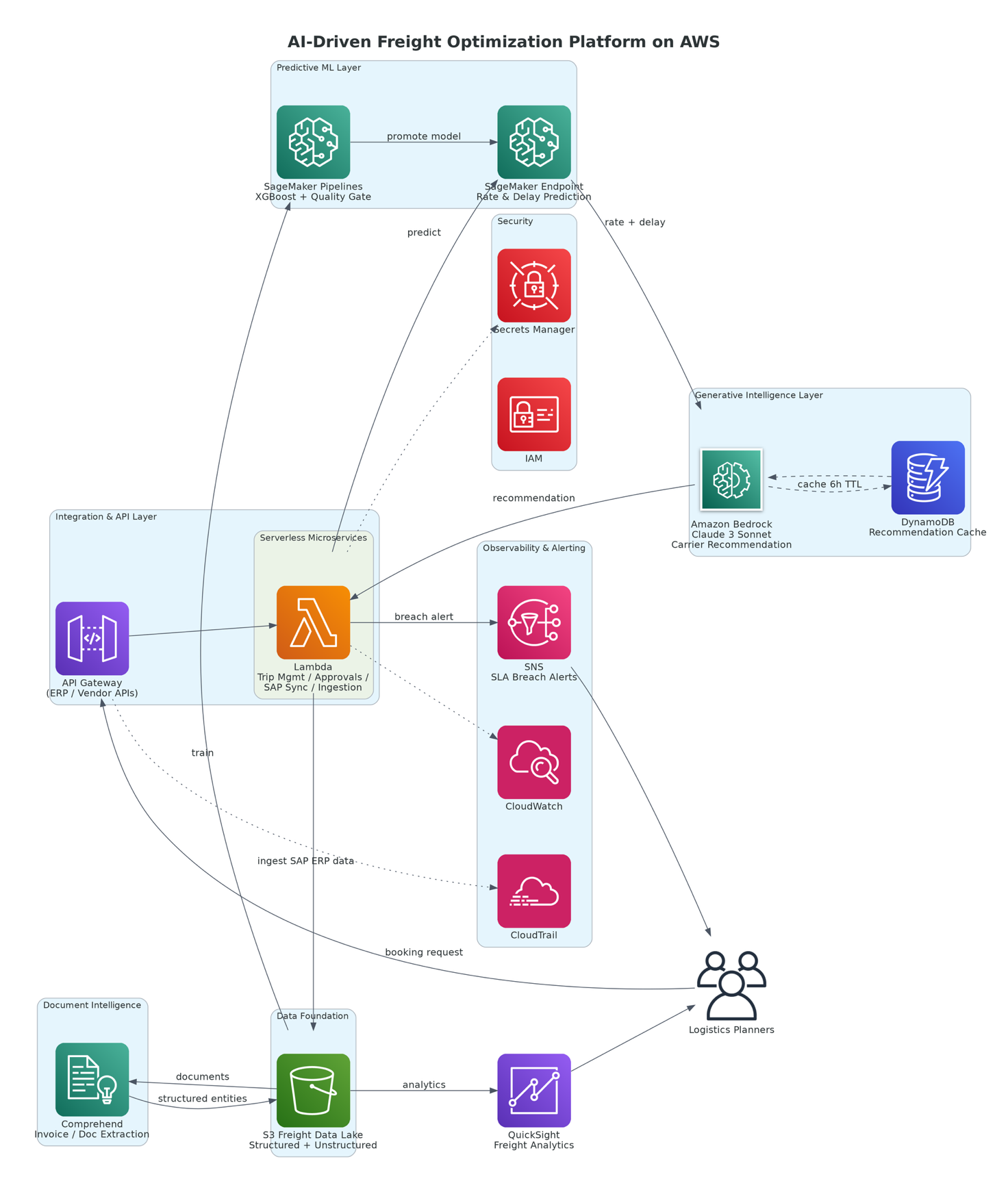
The architecture was designed around five principles: Data Lake First, Predictive ML + Generative AI Hybrid, Event-Driven Microservices, API-First Vendor and ERP Integration, and Continuous Learning Feedback Loop.
Key Architectural Decisions
These are the decisions that shaped the platform — and the reasoning behind each one.
Decision 1: Why a Hybrid ML + GenAI Pattern Instead of GenAI Alone?
When generative AI became widely available via Amazon Bedrock, the first question from the business was: "Can we just ask the AI what carrier to use?" It's a reasonable question. The answer is that LLMs alone are unreliable for logistics decisions because they have no access to your vendor's actual SLA history, your current rate contracts, or your specific route performance data.
The architecture separates the two responsibilities deliberately:
| Layer |
Technology |
Responsibility |
| Prediction |
Amazon SageMaker (XGBoost) |
What will the rate be? What is the delay probability? |
| Reasoning |
Amazon Bedrock (Claude 3 Sonnet) |
Given those predictions, what should the planner do? |
SageMaker produces deterministic, data-grounded outputs. Bedrock converts those outputs into contextual recommendations that a planner can act on. Neither layer works as well alone as they do together.
The business decision: GenAI without grounding produces hallucinated confidence. ML without reasoning produces numbers nobody acts on. The hybrid pattern produces decisions — which is what the business actually needed.
Decision 2: Why Amazon Bedrock Over a Self-Hosted LLM or Third-Party API?
We evaluated three options before selecting Bedrock:
- Self-hosted open-source LLM (Llama 2 on EC2) — lower per-token cost at scale, but required GPU instance management, security patching, model versioning, and a dedicated ML platform engineering capability the logistics team did not have. The total cost of ownership over 12 months exceeded Bedrock's pricing when engineering time was included.
- OpenAI API — strong output quality but introduced data residency concerns for India-based operations, no native AWS IAM integration, and required managing an external API dependency outside the existing AWS governance model.
- Amazon Bedrock — serverless inference with no infrastructure management, native VPC endpoint support, IAM-controlled access with full CloudTrail audit logging, and data that never leaves the AWS environment. The per-call cost at our volume (~6,500 bookings/month) was approximately $72/month — a marginal number against the freight savings.
The business decision: For an enterprise handling freight data involving vendor contracts and commercial terms, data residency and auditability are non-negotiable. Bedrock was the only option that met both requirements without operational overhead.
Decision 3: Why Invest in SageMaker Pipelines for Retraining Instead of a Static Model?
Freight economics are dynamic. Carrier rates change with fuel prices. Vendor reliability shifts with their own capacity constraints. Seasonal patterns vary year over year. A model trained on 18-month-old data will drift — and in a direction that makes it confidently wrong rather than obviously uncertain.
We built an automated retraining pipeline in SageMaker Pipelines that triggers on new completed-trip data, evaluates the candidate model against a quality gate, and only promotes models that meet the RMSE threshold. The model is always learning from the most recent freight outcomes.
The business decision: A static model is a depreciating asset. Automated retraining keeps the model current without requiring a data scientist to manually intervene every quarter — which, in practice, means it actually gets done.
Implementation Pattern
Data Foundation: Amazon S3 as the Freight Data Lake
The platform begins with data consolidation. We structured the S3 data lake with two zones:
- Structured data: trip logs, freight rate history, booking records, vendor SLA metrics — ingested from SAP ERP via Lambda-based extraction jobs
- Unstructured data: invoices (PDF), shipping documents, scanned paperwork — stored for Comprehend-based processing
Without a centralized data foundation, neither ML training nor GenAI grounding is possible. This was the first deliverable of the project, and the work that unlocked everything else.
Predictive Layer: SageMaker Pipeline with Quality Gate
PYTHON
import sagemaker
import boto3
from sagemaker.workflow.pipeline import Pipeline
from sagemaker.workflow.steps import TrainingStep
from sagemaker.workflow.condition_step import ConditionStep
from sagemaker.workflow.conditions import ConditionLessThanOrEqualTo
from sagemaker.workflow.functions import JsonGet
from sagemaker.inputs import TrainingInput

region = boto3.Session().region_name
role = sagemaker.get_execution_role()
bucket = "freight-data-lake-bucket"

xgb_estimator = sagemaker.estimator.Estimator(
    image_uri=sagemaker.image_uris.retrieve("xgboost", region, "1.7-1"),
    instance_type="ml.m5.xlarge",
    instance_count=1,
    output_path=f"s3://{bucket}/freight-model/output",
    role=role,
    hyperparameters={
        "max_depth": 5,
        "eta": 0.1,
        "objective": "reg:squarederror",
        "num_round": 300,
        "subsample": 0.8,
        "colsample_bytree": 0.8,
        "min_child_weight": 5,
    }
)

training_step = TrainingStep(
    name="FreightRateTraining",
    estimator=xgb_estimator,
    inputs={
        "train": TrainingInput(
            s3_data=f"s3://{bucket}/freight-data/train/",
            content_type="text/csv"
        ),
        "validation": TrainingInput(
            s3_data=f"s3://{bucket}/freight-data/validation/",
            content_type="text/csv"
        )
    }
)

# Only promote model if RMSE is within acceptable threshold
quality_gate = ConditionStep(
    name="CheckModelQuality",
    conditions=[
        ConditionLessThanOrEqualTo(
            left=JsonGet(
                step_name="EvaluateModel",
                property_file="evaluation",
                json_path="regression_metrics.rmse.value"
            ),
            right=0.08
        )
    ],
    if_steps=[model_register_step],
    else_steps=[notify_failure_step]
)

pipeline = Pipeline(
    name="FreightOptimizationPipeline",
    steps=[preprocessing_step, training_step, evaluation_step, quality_gate]
)
pipeline.upsert(role_arn=role)
Feature engineering enriched raw freight records with 34 input variables including rolling 30/60/90-day vendor SLA scores, route-level seasonal price indices, cargo weight-to-volume ratio, lead time delta, and peak season indicators. SHAP analysis via SageMaker Clarify revealed that vendor SLA history and lead time delta contributed over 38% of predictive weight — a finding that influenced how we structured vendor performance monitoring downstream.
Model performance:
| Metric |
Baseline (Rule-Based) |
XGBoost Model |
| Rate prediction error (MAPE) |
±19.3% |
±6.1% |
| Delay prediction accuracy |
Not available |
83% |
| Booking window optimization |
Manual (planner judgment) |
Automated |
| Endpoint inference time |
Not applicable |
~180ms average |
Generative Intelligence Layer: Bedrock Integration with Caching
PYTHON
import boto3, json, hashlib, time

bedrock = boto3.client("bedrock-runtime", region_name="ap-south-1")
dynamodb = boto3.resource("dynamodb", region_name="ap-south-1")
cache_table = dynamodb.Table("FreightRecommendationCache")

def generate_freight_recommendation(ml_output: dict) -> dict:
    # Cache key on inputs that meaningfully affect the recommendation
    cache_key = hashlib.md5(
        f"{ml_output['origin']}|{ml_output['destination']}|"
        f"{ml_output['cargo_type']}|{round(ml_output['predicted_rate'], -2)}|"
        f"{ml_output['lead_time_bucket']}"
        .encode()
    ).hexdigest()

    cached = cache_table.get_item(Key={"cache_key": cache_key}).get("Item")
    if cached:
        return json.loads(cached["recommendation"])

    prompt = f"""You are a freight logistics advisor for an industrial enterprise.

Context:
- Origin: {ml_output['origin']}
- Destination: {ml_output['destination']}
- Cargo type: {ml_output['cargo_type']}
- Weight: {ml_output['weight_kg']} kg
- Predicted freight rate: INR {ml_output['predicted_rate']:,.0f}
- Delay probability: {ml_output['delay_probability']}%
- Vendor SLA scores (top 3): {ml_output['vendor_scores']}
- Available lead time: {ml_output['lead_time_hours']} hours

Task:
1. Recommend the optimal vendor and vehicle type (FTL vs PTL) with rationale.
2. Suggest the best dispatch window to minimize cost and delay risk.
3. Flag any risk factors requiring manager escalation.
4. Write a 2-sentence approval summary for the logistics planner.

Respond as a JSON object with keys: vendor_recommendation, vehicle_type,
dispatch_window, risk_flags (array), approval_summary."""

    response = bedrock.invoke_model(
        modelId="anthropic.claude-3-sonnet-20240229-v1:0",
        contentType="application/json",
        accept="application/json",
        body=json.dumps({
            "anthropic_version": "bedrock-2023-05-31",
            "max_tokens": 512,
            "temperature": 0.2,
            "messages": [{"role": "user", "content": prompt}]
        })
    )

    result = json.loads(response["body"].read())
    recommendation = result["content"][0]["text"]

    # Cache for 6 hours — lane conditions don't change minute to minute
    cache_table.put_item(Item={
        "cache_key": cache_key,
        "recommendation": recommendation,
        "ttl": int(time.time()) + 21600
    })

    return json.loads(recommendation)
Bedrock latency averaged 1.6–2.4 seconds per call — acceptable for an asynchronous approval workflow. The DynamoDB cache reduced Bedrock calls by approximately 22% on high-frequency lanes where the same origin-destination-cargo combinations repeat on known patterns.
Document Intelligence: Amazon Comprehend
Logistics operations are document-heavy — invoices, shipping manifests, delivery receipts. We used Amazon Comprehend custom entity recognition to extract structured data from these documents automatically: vendor names, amounts, line items, and freight reference numbers. This eliminated manual data entry from the invoice reconciliation workflow and reduced document processing errors that had been causing downstream booking discrepancies.
Event-Driven Workflow Layer
The operational layer was built using API Gateway + Lambda microservices handling trip creation, booking approval, vendor notification, and SAP ERP synchronization. Lambda's stateless execution model meant the platform scaled naturally during peak booking windows — a period that had previously required the planning team to work overtime and still created approval backlogs.
Cost Architecture and AWS Service Spend
At steady-state processing approximately 6,500 freight bookings per month:
| Service |
Usage |
Estimated Monthly Cost |
| Amazon SageMaker |
2 × ml.m5.xlarge endpoints (24×7), ~12 pipeline runs/month |
~$332 |
| Amazon Bedrock (Claude 3 Sonnet) |
~6,500 calls, avg 800 input + 400 output tokens |
~$72 |
| Amazon Comprehend |
~18,000 document units (invoices, shipping docs) |
~$2 |
| AWS Lambda |
~420K invocations, 512MB memory |
~$5 |
| Amazon S3 |
~1.8 TB stored, ~200 GB monthly ingress |
~$42 |
| Amazon API Gateway |
~850K REST API calls |
~$3 |
| CloudWatch, SNS, Secrets Manager |
Monitoring, alerts, credential management |
~$24 |
| Total |
|
~$480/month |
SageMaker real-time endpoints running 24×7 are the single largest cost driver at approximately $168 per endpoint per month (ml.m5.xlarge at $0.23/hr). For batch-oriented routes where planners review recommendations in morning queues rather than on-demand, we migrated to asynchronous inference, reducing endpoint hours by approximately 40% and saving around $135/month without any impact on planner experience.
Against estimated annual freight savings of $2.8M–$3.2M on an approximately $17M annual freight spend (18% cost reduction), the platform infrastructure delivers over 480× ROI on AWS cost — not including the productivity recovery from 12 FTEs redirected from coordination to strategic procurement work.
Common Pitfalls (Real Lessons)
| Pitfall |
What Happened |
How We Fixed It |
| Model trained without vendor SLA features |
Predictions were accurate on rate but missed delay risk entirely |
Added vendor SLA rolling averages as first-class features in V2 |
| Bedrock called on every booking event |
Response latency created planner frustration during peak windows |
Added async workflow pattern + DynamoDB cache for repeat lanes |
| SageMaker endpoint always-on for low-traffic routes |
Cost inefficiency on routes with <5 bookings/week |
Migrated low-frequency routes to async inference endpoints |
| Comprehend custom model retrained infrequently |
New invoice formats from vendors broke entity extraction |
Added automated retraining trigger on document parsing error rate threshold |
Each of these emerged in production, not in testing. The operational feedback loop that feeds failures back into model and pipeline improvements is not optional — it is the mechanism that keeps the platform reliable over time.
Business Outcomes
| Metric |
Before |
After |
Business Impact |
| Freight cost vs. benchmark |
20–25% above |
Within 3–5% |
~$2.8M–$3.2M annual savings |
| Booking cycle time |
4 days |
< 24 hours |
Faster supply chain response |
| On-time delivery |
~78% |
97% |
Reduced customer SLA penalties |
| Booking approvals |
Manual, multi-step |
AI-assisted, single-step |
Planner capacity freed |
| FTE redeployment |
12 FTEs on coordination |
Redirected to strategic procurement |
Higher-value work per head |
| Audit trail |
None |
Full CloudTrail logging |
Compliance-ready |
The largest improvement came not from automation alone, but from the shift to data-driven decision-making. Planners who previously spent their time coordinating approvals now spend it analyzing vendor performance trends and negotiating better contracts — work that compounds over time in ways that automation cannot.
Lessons for Technology Leaders
- AI without data consolidation fails — The S3 data lake was the first and most important deliverable. Every model, every recommendation, and every insight runs on the quality of the underlying data. Teams that try to skip this step end up with impressive demos and unreliable production systems.
- The hybrid ML + GenAI pattern solves the last-mile problem — ML gives you predictions. GenAI gives you decisions. Neither is sufficient alone for operational use cases where humans need to act on the output.
- Continuous retraining is not optional in dynamic markets — Freight economics change frequently. A model trained six months ago is already working with stale assumptions. Automated retraining pipelines are not a nice-to-have — they are the mechanism that keeps the platform valuable.
- Observability must be designed in, not added later — CloudTrail, CloudWatch dashboards, and SNS alerting were built into the architecture from day one. Retrofitting observability onto a live production system is significantly more disruptive and always less complete.
- The ROI conversation is not about infrastructure cost — The business case for this platform is not the AWS bill. It is the $2.8M in freight savings, the 12 FTEs redirected to higher-value work, and the supply chain responsiveness that was impossible before. Frame the conversation that way and funding follows.
About the Author
Chandni Gadhvi is Program Manager – Data and AI at AeonX Digital Technology Limited, where she leads the architecture and delivery of cloud-native AI solutions for enterprise operations. She specializes in building intelligent, event-driven systems on AWS that convert operational data into business decisions. She is an advocate for data-first AI strategy and shares technical thought leadership to help engineering leaders move from pilot to production on AWS.